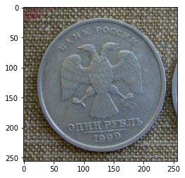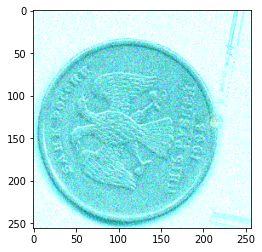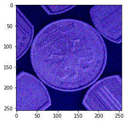
This is the 4th tutorial dedicated to coins classification. So far we were using the same approach: transfer learning CNN. And here we go again, we use it for classifying coins by year.
So why don't we classify it all in one pass: head-or-tail, value and year? All it takes is having a classifier with combined outputs, right?
The reason is, we don't have large (and clean) enough dataset. Even with my 20K+ images, it will suffer for some years as there were only limited minting that year ans I only have few images. So if I break them additionally for side/value/year... The net will undertrain.
The second reason is, we are NOT classifying coins yet! What we do is building a dataset for a "real" training! That's right, all we did so far, including current tutorial is sorting out a huge heap of images I got (automatically) from online, and marking them, assigning labels. To train a network for classification by values, we need, say, 100 images per coin. So a human (who else?) have to select about 400 images (1R, 2R, 5R, 10R). But if we wanted to train a net for value AND year, we would have to select, ideally, 100 coins per each year and value, which is 2000 images (Russian coins were chosen for this task because they have relatively short history, from 1997, but still, it is about 20 years).
So as you see, it is easier (not for network, but for a human tuning it) to classify it class-by-class.
Ideally, when we are done with this data preparation pipeline, we should be able to pick ANY coins images from ANY online sources, without paying any attention to their labels, and sort them to fit our dataset or throw them away. It will give us a larger dataset, which is exactly what we are after.
Finally, let's get clear on why do we need that huge dataset if by that point we already have a classifier? Well, our classifier can tell you "this is 1997 1Rouble coin". You don't need a computer to do exactly that!
What we are really after, is a classifier capable of finding rare and valuable versions of coins, something like "this is 1997 1R coin of a rare (0.05%) type, priced approx. 1000 roubles per new coin. To do it, we will have to find enough of different images of those rare versions of coins. If it is 0.05%, then to get 100 images we need 100*100/0.05 = 200000 of 1 rouble images. Is that possible, even with the Internet as a source? Probably no.
However, there is an alternative way, that will be describet in the latest tutorials. It still requires images, but not nearly that much.
Finally, the third reason we need that pipeline capable of getting images from the online mess. As time passes, new coins are minted, year after year. So either we will have to download them manually every year, clean them up and sort them before we retrain our nets, or we do it in a nice and automated way. That's what we are after.
As you can see, this code is very close to the code from the previous tutorial, the difference is mostly in inputs and outputs.
Same way as before, we are going to use Google Colab environment, taking the advantage of a free video card they grant us an access to. We will store data on a Google Drive, so first thing we need is to allow Colab to access the Drive:
from google.colab import drive
drive.mount("/content/drive/", force_remount=True)
Same way as we did in the second tutorial, we are going to use the transfer learning approach: we will load a pretrained EfficientNet and modify it to work on our task.
!pip install -q efficientnet
import efficientnet.tfkeras as efn
Next, i usually have a large "include" section, please note that some files may be included that are not really used: feel free to delete them:
import numpy as np
from sklearn.utils import shuffle
import pandas as pd
import tensorflow as tf
from tensorflow import keras
from tensorflow.keras import layers
import sys
import random
import matplotlib.pyplot as plt
import os
from os import listdir
from os.path import isfile, join
import json
from tensorflow.keras import regularizers
from tensorflow.keras.optimizers import Adamax
from tensorflow.keras.preprocessing.image import ImageDataGenerator
from tensorflow.keras.preprocessing.image import array_to_img, img_to_array
from tensorflow.keras import backend as K
from tensorflow.keras.applications.vgg16 import VGG16,preprocess_input
from tensorflow.keras.applications import InceptionResNetV2
from tensorflow.keras.applications import Xception, NASNetLarge
from mpl_toolkits.mplot3d import Axes3D
from sklearn.manifold import TSNE
from tensorflow.keras.layers import Input, Conv2D, MaxPooling2D
from tensorflow.keras.layers import Dense, Activation, Dropout
from tensorflow.keras.layers import Flatten, Lambda, concatenate
from tensorflow.keras.layers import BatchNormalization, GlobalAveragePooling2D
from tensorflow.keras.callbacks import LambdaCallback
from tensorflow.keras.callbacks import ModelCheckpoint
from tensorflow.keras.models import Sequential
from sklearn.neighbors import NearestNeighbors
import seaborn as sns
import cv2
from tensorflow.python.keras.utils.data_utils import Sequence

import re
Let's see which version of Tensorflow is used. This step is important, as Google is known for suddenly changing (increasing) versions:
import tensorflow as tf
print(tf.__version__)
tf.test.gpu_device_name()
The output in my case was:
2.4.0
'/device:GPU:0'
Folders we are going to use in our project
working_path = "/content/drive/My Drive/04_coin_year/"

best_weights_filepath = working_path + "models/04_coin_value_best.h5"
last_weights_filepath = working_path + "models/04_coin_value_last.h5"
As we save our last training configuration, we don't have to redo training every time we start the notebook: we can simply reload from disk:
bDoTraining = True
We are going to scale down images to 224x224, use batch size 8 during training, and so on: here are constants we will need. Names are self-explainatory. We are also going to break our data to training images (used to tune network's weights), validation images used to calculate performance on data the net never saw) and the rest (testing data, used to test the result).
IMAGE_SIZE = 224 # size for Efficient Net B0
input_shape=(IMAGE_SIZE, IMAGE_SIZE, 3)

BATCH_SIZE = 8

alpha = 0.4

TRAINING_IMAGES_PERCENT = 0.6
VALIDATION_IMAGES_PERCENT = 0.2

IMAGE_ROTATION_ANGLE = 180
Classes our classifier should distinguish. Note that, unlike in step 2, it is not a binary classifier, so we use the one-hot encoding, provided by Pandas library.
Note: our plan is to build a classifier. To do it, I (human) have created one folder per each year and copied couple of images of corresponding coins there. When we are done classifying, we will combine classification data (year of a particular coin) with coin value data for the same coin, that were obtained during the previous step. This way we can create a combined year - value folder structure.
# Classes our classifier should distinguish
arrClasses = ["1997", "1998", "1999", "2000", "2001",
  "2002", "2003", "2004", "2005", "2006", "2007", "2008",
  "2009", "2010", "2011", "2012", "2013", "2014", "2015",
  "2016", "2017", "2018", "2019"]

# Note that coin value is not an output of our network. We only use it at final testing, to access folders
# crearted by a value classifier on the previous step (prev. tutorial).
arrValues = ["1R", "2R", "5R", "10R"]

pdClassLabels = pd.get_dummies(arrClasses)
In the previous tutorials we had no choice but to physically move images around. We have downloaded images from the net, and we had a lot of junk there. We did cropping which could easily make ten images out of one, if that one contained 10 coins. We groupped images to pairs (head/tail) and removed images that had no pair. However for our current task, we already have images we need, and all we have to do is placing labels on them, so to speak. As the result, instead of copying images from "source" location to a "target" one (for example, to "1Rub/2Rub etc folders), we will create a file containing labels, describing existing images. This approach saves a lot of disk space.
# We are going to store labeled data for training in the following format:
# arrLabeledData = [ { 'id':'169860023_00_00_head.png', 'class':'1R' }, ... ]

def scanCoinsDir(strDirName):
  path = working_path + "images/" + strDirName
  arrImageNames = [f for f in os.listdir(path)] # if f.endswith('.txt')]
  for file_name in arrImageNames:
    arrLabeledData.append({ 'id': file_name, 'year': strDirName})

# ---

np.random.seed(7)

if(bDoTraining):
  arrLabeledData = []

  for strDirName in arrClasses:
    scanCoinsDir(strDirName)

  np.random.shuffle(arrLabeledData)
Function to load images:
def loadImage(path):
    img=cv2.imread(str(path))
    img = cv2.resize(img, (IMAGE_SIZE, IMAGE_SIZE))
    img = cv2.cvtColor(img, cv2.COLOR_BGR2RGB)
    img = img.astype(np.float32)/255.
    img = img.reshape(input_shape)

    return img
It is always a good idea to make sure everything works as intended, so let's test image loading:
if(bDoTraining):
  nImageIdx = random.randint(0, len(arrLabeledData))

  print(arrLabeledData[nImageIdx])

  img = loadImage(join(working_path, "images/", arrLabeledData[nImageIdx]['year'], arrLabeledData[nImageIdx]['id']))
  #img = img.reshape((IMAGE_SIZE, IMAGE_SIZE))
  plt.imshow(img)
  plt.show()

> {'id': '137268312_000_00_tail.png', 'year': '1999'}

When doing classification on images, we have a choice. Our coins are randomly rotated. On one side it is good, we can even rotate them additionally, to make it harder for a network to overtrain. Or we can align images, arguing that it is easier to learn classification task on images with the same orientation (size, color palette etc). We are going to choose the first approach: we will do so called image augmentation: size, rotation and so on can be randomly altered, so that the network learns to generalize, rather than just memorizing images of the training set (and therefore performing poorly on images it never saw). Particularly, we are going to try adding random noise to images:
Additionally, as we NEED diverse images, we are going to add some more functionality to make images different:
def add_noise(img):
    VARIABILITY = 60
    deviation = VARIABILITY*random.random() / 255.
    noise = np.random.normal(0, deviation, img.shape)
    img += noise
    np.clip(img, 0., 1.)
    return img

def shiftColors(img):
    hsv = cv2.cvtColor(img, cv2.COLOR_BGR2HSV)
    h, s, v = cv2.split(hsv)

    value = (0.5 - np.random.randint(255) / 255.)

    lim = 1. - value
    v[v > lim] = 1.
    v[v <= lim] += value

    final_hsv = cv2.merge((h, s, v))
    img = cv2.cvtColor(final_hsv, cv2.COLOR_HSV2BGR)

    return img

def shiftChannelColors(img):
    value_r = (0.5 - np.random.randint(255) / 255.)
    value_g = (0.5 - np.random.randint(255) / 255.)
    value_b = (0.5 - np.random.randint(255) / 255.)

    lim_r = 1. - value_r
    lim_g = 1. - value_g
    lim_b = 1. - value_b

    img[..., 0][value_r > lim_r] = 1.
    img[..., 1][value_g > lim_g] = 1.
    img[..., 2][value_b > lim_b] = 1.

    img[..., 0][value_r <= lim_r] += value_r
    img[..., 1][value_g <= lim_g] += value_g
    img[..., 2][value_b <= lim_b] += value_b

    return img
To perform the above mentioned image augmentation, let's use the image data generator provided with TF:
if(bDoTraining):
  datagen = ImageDataGenerator(
    samplewise_center=True,
    rotation_range=IMAGE_ROTATION_ANGLE,
    width_shift_range=0.1,
    height_shift_range=0.1,
    zoom_range=[1.0, 1.2]
  )
The following function is used to get an image by index from data we loaded earlier, using image data generator we just created:
def getImage(nImageIdx, datagen, bIsTrain):
  img = loadImage(join(working_path, "images/", arrLabeledData[nImageIdx]['year'], arrLabeledData[nImageIdx]['id']))

  arrImg = img_to_array(img)
  #if(bIsTrain):
  arrImg = datagen.random_transform(arrImg) # augmentation
  arrImg = add_noise(arrImg)
  arrImg = shiftChannelColors(arrImg)

  return np.array(arrImg, dtype="float32")
Again, we need to make sure everything works, so let's see what this function returns:
if(bDoTraining):
  nImageIdx = 0#np.random.randint(len(arrLabeledData))

  img = getImage(nImageIdx, datagen, True)

  plt.imshow(img) #, cmap='gray')
  plt.show()

Most likely, we will not be able to make our code perfect first time we run it. So we need to be able to delete networks we have saved on previous attempts, ones with non-optimal parameters and so on.
def deleteSavedNet(weights_filepath):
    if(os.path.isfile(weights_filepath)):
        os.remove(weights_filepath)
        print("deleteSavedNet():File removed")
    else:
        print("deleteSavedNet():No file to remove")
Generally, we either need to use a Keras-provided callback to plot charts as we train the network, or (better) use TensorBoard. However, the current task is rather simple, so we'll simply wait for the training to finish, and only then wisplay charts:
def plotHistory(history, strParam1, strParam2):
	plt.plot(history.history[strParam1], label=strParam1)
	plt.plot(history.history[strParam2], label=strParam2)
	plt.legend(loc="best")
	plt.show()

def plotFullHistory(history):
    arrHistory = []
    for i,his in enumerate(history.history):
        arrHistory.append(his)
    plotHistory(history, arrHistory[0], arrHistory[2])
    plotHistory(history, arrHistory[1], arrHistory[3])
Now a function that creates a model. It loads the EfficientNet, removes its last layers (the classifier) and attaches our own classifier, one we are going to train:
def createModel(nL2, dDrop, optimizer):
  inputs = keras.Input(shape=(IMAGE_SIZE, IMAGE_SIZE, 3))

  model_b0 = efn.EfficientNetB0(weights='imagenet',
	include_top=False)(inputs)
  model_b0.trainable = False

  model_concat = model_b0

  model_classifier = layers.Flatten(name="Flatten")(model_concat)

  model_classifier = layers.Dense(32, kernel_regularizer=regularizers.l2(nL2),
	activation='relu', name="Dense128")(model_classifier)
  model_classifier = layers.LeakyReLU(alpha=0.1, name="LeakyReLU")(model_classifier)
  model_classifier = layers.Dropout(dDrop, name="Dropout")(model_classifier)

  base_model = layers.Dense(len(arrClasses), activation="softmax",
	kernel_regularizer=regularizers.l2(nL2), name="DenseEmbedding")(model_classifier)

  model = keras.Model(inputs=inputs, outputs=base_model, name="embedding_model")

  model.compile(loss=keras.losses.CategoricalCrossentropy(),
	optimizer=optimizer, metrics=["accuracy"])

  return model
TF ver 2 have some problems with old style image data generators. Instead, it offers us the new approach that uses Sequence-derived classes. On one side, this approach takes more efforts then just providing generators to a training function. On the other - it handles parallel tasks (or so they tell us) and is, therefore, faster. Here is the Sequence-derived generator we are going to use in our code:
def getStepSizes():
    nNumOfSamples = len(arrLabeledData)
    nNumOfTrainSamples = nNumOfSamples * TRAINING_IMAGES_PERCENT
    nNumOfValidSamples = nNumOfSamples * VALIDATION_IMAGES_PERCENT

    step_train = nNumOfTrainSamples // BATCH_SIZE

    nNumOfValidSamples = int(nNumOfTrainSamples * VALIDATION_IMAGES_PERCENT / TRAINING_IMAGES_PERCENT)
    step_valid = nNumOfValidSamples // BATCH_SIZE

    if(step_train < 100):
      step_train = 100

    if(step_valid < 100):
      step_valid = 100

    return (step_train, step_valid)
The following class is used to produce batches of images (and labels) that are used during training. Sequence class that is used as a parent is a new standard of Keras (if you don't want to use tfdata), it is highly paralelizeable and convenient:
class MyImageDataGenerator(Sequence):
  def __init__(self, bIsTrain):
    self.batch_size = BATCH_SIZE
    self.bIsTrain = bIsTrain

    nNumOfSamples = len(arrLabeledData)

    step_train, step_valid = getStepSizes()
    if(bIsTrain):
      self.nStartIdx = 0
      self.nEndIdx = nNumOfSamples * TRAINING_IMAGES_PERCENT - 1
      self.STEP_SIZE = step_train
    else:
      self.nStartIdx = nNumOfSamples * TRAINING_IMAGES_PERCENT
      self.nEndIdx = nNumOfSamples * (TRAINING_IMAGES_PERCENT + VALIDATION_IMAGES_PERCENT) - 1
      self.STEP_SIZE = step_valid

    print("STEP_SIZE: ", self.STEP_SIZE, " (bIsTrain: ", bIsTrain, ")")

  def __len__(self):
    return self.STEP_SIZE

  def __getitem__(self, idx):
    arrBatchImages = []
    arrBatchLabels = []

    for i in range(self.batch_size):
      nImageIdx = np.random.randint(self.nStartIdx, self.nEndIdx)
      sample = arrLabeledData[nImageIdx]

      img = getImage(nImageIdx, datagen, self.bIsTrain)
      strLabel = sample['year']

      arrBatchImages.append(img)
      arrBatchLabels.append(pdClassLabels[strLabel].to_list())

    return np.array(arrBatchImages), np.array(arrBatchLabels)
Now we create generators for training and validation:
if(bDoTraining):
  gen_train = MyImageDataGenerator(True)
  gen_valid = MyImageDataGenerator(False)
Same way as for all image processing routines, let's make sure everything works:
def ShowImg(img, label):

  print(label)

  fig = plt.figure()
  fig.add_subplot(1, 1, 1)
  plt.imshow(img) #, cmap='gray')
  plt.show()
  plt.close()

# And test it:
if(bDoTraining):
  (images, labels) = gen_valid.__getitem__(0) #next(gen_train)

  for i, img in enumerate(images):
    ShowImg(img, labels[i])
    break

As we do training, we need to perform certain actions at certain moments. For example, we want to save the current (last) and the best (one with minimum error) networks at the end of each epoch.
def getCallbacks(monitor, mode, model):
	checkpoint = ModelCheckpoint(best_weights_filepath,
		monitor=monitor, save_best_only=True,
		save_weights_only=True, mode=mode, verbose=1)

	save_model_at_epoch_end_callback =
		LambdaCallback(on_epoch_end=lambda epoch,
		logs: model.save_weights(last_weights_filepath))

	callbacks_list = [checkpoint, save_model_at_epoch_end_callback]

	return callbacks_list
The following function will load the previously saved model, if it was saved, of course. Depending on the bBest flag that we pass to it, it loads either best or last model. Best one is used after the training is complete, to actually USE the resulting network. The last network is used in case our training was interrupted, so we can resume it from a checkpoint, rather than starting from the very beginning.:
def loadModel(model, bBest):
  if(bBest):
    path = best_weights_filepath
    strMessage = "load best model"
  else:
    path = last_weights_filepath
    strMessage = "load last model"

  if(os.path.isfile(path)):
    model.load_weights(path)
    print(strMessage, ": File loaded")
  else:
    print(strMessage, ": No file to load")

  return model
The following function is used to do training. Depending on parameters we pass, it deletes (or not) the previously saved network, creates a model, loads the previously saved results (if we haven't deleted them earlier). After the training is complete, it plots the charts of training and testing errors.
def trainNetwork(EPOCHS, nL2, nDrop, optimizer, history, bCumulativeLearning = False):

  if(bCumulativeLearning == False):
    deleteSavedNet(best_weights_filepath)

  random.seed(7)

  model = createModel(nL2, nDrop, optimizer)
  print("Model created")

  callbacks_list = getCallbacks("val_accuracy", 'max', model)

  if(bCumulativeLearning == True):
    loadModel(model, False)

  STEP_SIZE_TRAIN, STEP_SIZE_VALID = getStepSizes()

  print(STEP_SIZE_TRAIN, STEP_SIZE_VALID)
  print("Available metrics: ", model.metrics_names)

  history = model.fit(gen_train,
    validation_data=gen_valid, verbose=1,
    epochs=EPOCHS, steps_per_epoch=STEP_SIZE_TRAIN,
    validation_steps=STEP_SIZE_VALID, callbacks=callbacks_list)

  print(nL2)
  plotFullHistory(history)

  # TBD: here, return best model, not last one
  return model, history
This function performs the actual training and calculates the accuracy of a resulting net:
def train_and_test(EPOCHS, nL2, nDrop, optimizer, learning_rate, bCumulativeLearning):
  model, history = trainNetwork(EPOCHS, nL2, nDrop, optimizer, bCumulativeLearning)
  print("loading best model")
  model = loadModel(model, True)

  return model
As the function train_and_test is just the function, it would not call itself, so we have to do it:
opt = tf.keras.optimizers.Adam(0.0002) ##Adamax(lr=0.0001,
	beta_1=0.9, beta_2=0.999, epsilon=None, decay=0.0)
nL2 = 0.6
nDrop = 0.6

if(bDoTraining):
  EPOCHS = 100
  learning_rate=0.001

  np.random.seed(7)
  model = train_and_test(EPOCHS, nL2, nDrop, opt,
	learning_rate, bCumulativeLearning=False)

  model = loadModel(model, True)
  model.save(best_weights_filepath)    # A full model is saved
A helper function to figure our where training ant test sets begin and end:
def getClassMinMax(bIsTrain):
  nLen = len(arrLabeledData)
  if(bIsTrain):
    nMinIdx = 0
    nMaxIdx = nLen * TRAINING_IMAGES_PERCENT - 1
  else:
    nMinIdx = nLen * TRAINING_IMAGES_PERCENT
    nMaxIdx = nLen * (TRAINING_IMAGES_PERCENT + VALIDATION_IMAGES_PERCENT) - 1

  return int(nMinIdx), int(nMaxIdx)
An additional test, which can be very useful when something is not right and we want to "see" the problem. Here we display test images along with predictions for them IF Prediction and Ground Truth are different:
if(bDoTraining):
  #model = createModel(nL2, optimizer)
  #model = loadModel(model, True)

  nMinIdx, nMaxIdx = getClassMinMax(False)

  for i, nImageIdx in enumerate(range(nMinIdx, nMaxIdx)):
    print(i+1, "of", nMaxIdx - nMinIdx)
    img = loadImage(join(working_path, "images/",
		arrLabeledData[nImageIdx]['year'], arrLabeledData[nImageIdx]['id']))

    arrImg = img_to_array(img)
    arrImg = np.array(arrImg, dtype="float32")

    # ---

    test_preds = model.predict(arrImg.reshape(1, IMAGE_SIZE, IMAGE_SIZE, 3))

    nIdx = test_preds.argmax()
    if(arrLabeledData[nImageIdx]['year'] != arrClasses[nIdx]):
      print("GT: ", arrLabeledData[nImageIdx]['year'], ";
		Pred: ", arrClasses[nIdx])
      plt.imshow(img)
      plt.show()
Finally, our network is production-ready. Now we can process our images, ALL of them Same as above in "test" section, but this time we process images from output folder of step 3.
Note that we don't have that much space on Colab, and our dataset is 26,000+ images. So instead of copying images of stage 3, we are going to index them.
About images_processed_remain: it has files sorted to head/tail WRONG. We can use it next time we train head/tail classifier.
images_source_path =
	"/content/drive/My Drive/03_coin_value/03_output/"

# We already have coins sorted by value.
# Now we want year - value (value is a subdir of year).

model = createModel(nL2, nDrop, opt)
model = loadModel(model, True)

arrOutput = []

print("Processing tails")

for strDirName in arrValues:
  arrSourceImageNames = [f for f in
	listdir(images_source_path + strDirName)]

  nTotal = len(arrSourceImageNames)

  for i, file_name in enumerate(arrSourceImageNames):
    if(i%100 == 0):
      print("Year ", strDirName, ": ", i, " of ", nTotal)

    # 169860023_00_00_tail(.png)
    # Here 169860023 is number of image set
	#     (groups of photos of a set of coins from meshok.ru)
    # First 00 is number of image (from meshok.ru, so they have
	#     169860023_00, 169860023_01...)
    # Second 00 is coin number within coin set
	# (image with 3 coins: 169860023_00_00, 169860023_00_01,
	#     169860023_00_02, turn coins, 169860023_01_00,
	#     169860023_01_01, 169860023_01_02)

	# For test can use short list:
	# # ['169860023_00_00_tail', 'png']
	word_list = file_name.split(".")

    image_name = word_list[0]
    image_ext = word_list[1]

    # Russian coins have year on "tail" side
    if("head" in image_name):
      continue

    # ["169860023", "000", "00", "tail"]
    image_name_parts = image_name.split("_")

    image_path = join(images_source_path, strDirName, file_name)
    img = loadImage(image_path)
  #  print("GT: ", arrLabeledData[nImageIdx]['class'],
  #      "; Pred: ", arrClasses[nIdx])
  #  plt.imshow(img)
  #  plt.show()

    arrImg = img_to_array(img)
    arrImg = np.array(arrImg, dtype="float32")

    # ---

    test_preds = model.predict(arrImg.reshape(1, IMAGE_SIZE, IMAGE_SIZE, 3))

    nIdx = test_preds.argmax()
    strClass = arrClasses[nIdx]

    # Find out if info for this coin
	# (but for other image of it) is in arrOutput

    # 'coin_id': coin set / image number within set
    # 'id': num. of image version (like we have 3 photos
	# where the same coin is coin number 7: xxxx_00_07,
	# xxxx_01_07, xxxx_02_07). Note: this is part of a sub-array
    # 'side': head/tail

    coin_id = image_name_parts[0] + "_" + image_name_parts[2]
    coin_info = [info for info in arrOutput if info['coin_id'] == coin_id]
    if coin_info:
      coin_info = coin_info[0]
      nMaxConfidence = test_preds[0][nIdx]

      # If classes predicted for different photos of the same
	  # coin are different, show that coin
      if(strClass != coin_info['class']):
        print("================\n", coin_info['class'],
			" vs ", strClass, "; Confidence: ",
			coin_info['confidence'], nMaxConfidence)
        if(nMaxConfidence < coin_info['confidence']):
          strClass = coin_info['class']
        plt.imshow(img)
        plt.show()

      coin_info['data'].append({'id': image_name_parts[1],
		'side':image_name_parts[3], 'ext': image_ext})
      coin_info['confidence'] = nMaxConfidence
      coin_info['class'] = strClass

    else:
      coin_info = { 'coin_id':coin_id,
		'data': [{'id': image_name_parts[1],
			'side':image_name_parts[3], 'ext': image_ext}],
			'value': strDirName,
			'year':strClass, 'confidence':test_preds[0][nIdx] }
      arrOutput.append(coin_info)
So far we used only "tail" images, as this is where Russian coins have their value minted. We need to add "head" images of corresponding coins to our results. We can do it, as head and tail images follow the same naming standard:
print(">>> Processing heads <<<")

for strDirName in arrValues:
  arrSourceImageNames = [f for f in
	listdir(images_source_path + strDirName)]

  for i, file_name in enumerate(arrSourceImageNames):

    if(i%100 == 0):
      print("Year ", strDirName, ": ", i, " of ", nTotal)

	# For test purposes can use a short list:
	# # ['169860023_00_00_tail', 'png']
    word_list = file_name.split(".")
    image_name = word_list[0]
    image_ext = word_list[1]

    # Russian coins have year on "tail" side,
	# so tails are already processed
    if("tail" in image_name):
      continue

    # ["169860023", "00", "00", "head"]
    image_name_parts = image_name.split("_")

    # ---

    # Find out if info for this coin (but for other image of it)
	# is in arrOutput. As we might have more than one "head",
	# we'll take 0th head class for this tail image

    coin_id = image_name_parts[0] + "_" + image_name_parts[2]
    coin_info = [info for info in arrOutput if info['coin_id'] == coin_id]

    if coin_info:
      coin_info = coin_info[0]
      coin_info['data'].append({'id': image_name_parts[1], 'side':image_name_parts[3] })
Finally, as an additional step, let's copy images to corresponding folders: 1997/, 1998/... Be careful, as it is possible to run out of Colab disk space.
for i, coin_info in enumerate(arrOutput):
  if(i%100 == 0):
    print(i, " of ", len(arrOutput))

  coin_id = coin_info['coin_id']
  year = coin_info["year"] # "1997"
  word_list = coin_id.split("_")  # 90970347, 00
  ext = "png"
  for data in coin_info['data']:
    id = data["id"]                 # "003"
    side = data["side"]             # "head"
    value = data["value"]

    strFileName = word_list[0] + "_" + id + "_"
		+ word_list[1] + "_" + side + "." + ext

    # Create target folder if it doesn't exist
    strTargetFolder = working_path + '04_output/'
		+ year + "/" + value + "/"

	print("Moving", images_source_path + strFileName, "to",
		strTargetFolder + strFileName)

#    if not os.path.exists(strTargetFolder):
#      os.makedirs(strTargetFolder)

    # Move file to target folder
#    if(os.path.exists(images_source_path + strFileName)):
#      os.rename(images_source_path + strFileName, strTargetFolder + strFileName)