Using synthetic dataset for copter detection
In this post we are going to perform the image segmentation detecting a single quadcopter (one quadcopter per image) using a simple CNN. This aproach has its advantages: it is way faster than more complex YOLO, SSD or Faster-RCNN approaches. All we need is to show the image to a network and to get quadcopter's coordinates as an output.
The post is intended to be more educational than practical: we are going to address an issue of dataset generation. After all, to train a NN, we need a lot of images, and in our case, it is going to be THE SAME quadcopter, in different rooms, and at different angles and distances. So... why don't we take two dosens of quadcopter images, and paste them, at different scales and spots, to photos of rooms? This way we can get nearly infinite amount of images for training!
As always, obvious advantages of a method are accompanied by the obvious disadvantages.
First of all, we can not have more than one quadcopter per image. It is ok, as we expected
so initially. Another problem is the size of a copter, related to the size of an image.
If the copter is far enough from the camera, it becomes too small for a CNN resolution.
For example, EfficientNet B0 is 224x224 pixels. if a copter occupies 1/10 of an image,
it will be only 22x22 px. Below, we'll try fixing the problem by using larger input sizes
(like B1 to B7), but at some point quality of our image recognition will stop improving.
The code below ia s fully functional example, so let's just go through it, looking at details.
As usual, we start with allowing Google Colab to access Google Drive:
from google.colab import drive
drive.mount("/content/drive/", force_remount=True)
Install EfficientNet in our system. We use so called "transfer learning" approach. Someone (Google) has already trained the EfficientNet on a huge dataset, so it can recognize cats, chairs and so on. It is of no use for quacopter detection by itself, however, it means this network has already seen a lot of graphical primitives, like lines, circles etc. So we will use it and just alter a bit, to train additionally on our quadcopter set. It will make the training process dramatically shorter and will - also dramatically - reduce requirements for the dataset size.
There are eight Efficient Nets, from EfficientNet0 to EfficientNet7, the difference is in the input (and overall) size. We use the following table (https://keras.io/examples/vision/image_classification_efficientnet_fine_tuning/) as a reference for those input sizes:
| Base model | resolution |
| EfficientNetB0 | 224 |
| EfficientNetB1 | 240 |
| EfficientNetB2 | 260 |
| EfficientNetB3 | 300 |
| EfficientNetB4 | 380 |
| EfficientNetB5 | 456 |
| EfficientNetB6 | 528 |
| EfficientNetB7 | 600 |
!pip install -q efficientnet
import efficientnet.tfkeras as efn
Import everything we need. I am sure some links are not required, but I was to lazy to find them and to comment them out:
import numpy as np
from sklearn.utils import shuffle
import pandas as pd
import tensorflow as tf
from tensorflow.keras import layers
import json
from tensorflow.keras.utils import Sequence
import sys
import random
import math
from copy import copy, deepcopy
import matplotlib.pyplot as plt
import matplotlib.patches as patches
import os
from os import listdir
from os.path import isfile, join
import json
from tensorflow.keras import regularizers
from tensorflow.keras.optimizers import Adamax
from tensorflow.keras.preprocessing.image import ImageDataGenerator
from tensorflow.keras.preprocessing.image import array_to_img, img_to_array
from tensorflow.keras import backend as K
from tensorflow.keras.applications.vgg16 import VGG16,preprocess_input
from tensorflow.keras.applications import InceptionResNetV2, Xception
from tensorflow.keras.applications import NASNetLarge
from mpl_toolkits.mplot3d import Axes3D
from sklearn.manifold import TSNE
from tensorflow.keras.layers import Input, Conv2D, MaxPooling2D
from tensorflow.keras.layers import Dense, Activation, Dropout
from tensorflow.keras.layers import Flatten, Lambda, concatenate
from tensorflow.keras.layers import BatchNormalization, GlobalAveragePooling2D
from tensorflow.keras.callbacks import LambdaCallback
from tensorflow.keras.callbacks import ModelCheckpoint
from tensorflow.keras.models import Model
from tensorflow.keras.models import Sequential
from sklearn.neighbors import NearestNeighbors
import seaborn as sns
import cv2
import re
Is GPU Working? Google provides us with access to their GPUs, and sometimes we forget turning this feature on:
import tensorflow as tf
print(tf.__version__)
tf.test.gpu_device_name()
I am going to save the last NN, just in case the training is interrupted, and the best NN - for a future use:
# Folders we are going to use in our project
working_path = "/content/drive/My Drive/copter_detect_my/"

best_weights_filepath = working_path + "models/copter_detect_best.h5"
last_weights_filepath = working_path + "models/copter_detect_last.h5"
The following boolean flag allows us to either train the NN, or load a previously trained one, if we want to do testing. As we save our last training configuration, we don't have to redo training every time we start the notebook: we can simply reload from disk.
bDoTraining = True
I am going to try few versions of EfficientNet (B0, B1, ...), so here are input sizes they accept, in no particular order. For a reference, see the table above. Also, when i select a particular size here, i have to change the type of a network below in CreateNN function:
# Constants for training and image preprocessing
IMAGE_SIZE_X = 380 #300 #260 #240 #224 #456 #512 #700
IMAGE_SIZE_Y = 380 #300 #260 #240 #224 #456 #683 #934
The larger the network, the higher are the chances that it will not fit in Colab's memory. As a simple countermeasure, we can reduce the size of a batch. Generally, we should try keeping the batch size as large as we can, it will improve training.
BATCH_SIZE = 4 #1
Now, the most important part: where are we going to get the images? We can, of course, make a large amount of photos, but it is time consuming. Instead, we take some small number of photos of quadcopters, taken by different angles. We clean them, making a background transparent. Then we paste them dynamically (meaning, we generate images on the fly), at different (random) scales to different random spots of photos of rooms.
First, let's load images of quadcopters. We keepthem in an array in memory, as there are just 37 images. Instead of coordinates (left - top - right - bottom), we keep center and radius:
copter_images_path = working_path + "images_copter/"

# Download annotations.json
with open(copter_images_path + 'annotations.json') as f:
    json_data = json.load(f)

# Scan json

arrCopterImageNames = []
arrCoordinates = []
arrCopterImages = []

file_info_json = json_data['_via_img_metadata']

for x in file_info_json:
  strImageFileName = file_info_json[x]['filename']

  shape = file_info_json[x]['regions'][0]['shape_attributes']
  copter_rect = [shape['x'], shape['y'], shape['width'], shape['height']]
  #print("%s:\r\n\t%s, %s" % (x, strImageFileName, copter_rect))

  # ---

  arrCopterImageNames.append(copter_images_path + strImageFileName)

  # Note that we are downloading a full-size image
  img_copter=cv2.imread(copter_images_path + strImageFileName,
	cv2.IMREAD_UNCHANGED)
  img_copter = cv2.cvtColor(img_copter, cv2.COLOR_BGRA2RGBA)

  arrCopterImages.append(img_copter)

  # Replace rect with center/radius
  copter_center_x = copter_rect[0] + (int)(copter_rect[2] / 2)
  copter_center_y = copter_rect[1] + (int)(copter_rect[3] / 2)

  copter_radius = (int)(max(copter_rect[2], copter_rect[3]) / 2)

  arrCoordinates.append([copter_center_x, copter_center_y, copter_radius])

# Shuffle, otherwise all negatives will go to validation set
arrCoordinates = np.array(arrCoordinates, dtype="float32")
arrCoordinates = np.array(arrCoordinates)

print(arrCopterImageNames)
print(arrCoordinates)
Then we load images of rooms:
arrAppartmentImageNames = []
arrAppartmentImages = []

appartment_images_path = working_path + "images_appartment/"

for strImageFileName in os.listdir(appartment_images_path):
  if strImageFileName.endswith('.jpg'):
    arrAppartmentImageNames.append(strImageFileName)
    img=cv2.imread(appartment_images_path + strImageFileName)
    img = cv2.cvtColor(img, cv2.COLOR_BGR2RGB)
    img = cv2.resize(img, (IMAGE_SIZE_X, IMAGE_SIZE_Y))
    arrAppartmentImages.append(img)

print(arrAppartmentImageNames)
Now, as we are going to rescale images as we combine them, we need to work with copies, not with items in the original array:
def loadCopterImage(nIdx):
  return arrCopterImages[nIdx].copy()

def loadAppartmentImage(nIdx):
  return arrAppartmentImages[nIdx].copy()
Let's test our loaders. It is a good idea, every time we write a function we can test, writing also a testing code (note that for loaders above it is not necessary, as we can see values in arrays using Colab's "run selection"):
# Let's test our loadImage() function, just to be sure it works properly
nImageIdx = random.randint(0, len(arrCopterImageNames) - 1)

print(arrCopterImageNames[nImageIdx])

img = loadCopterImage(nImageIdx)

figure, ax = plt.subplots(1)
circle = patches.Circle((arrCoordinates[nImageIdx][0],
  arrCoordinates[nImageIdx][1]),
  arrCoordinates[nImageIdx][2],
  linewidth=2, edgecolor='r', facecolor="none")
ax.imshow(img)
ax.add_patch(circle)
plt.show()

Similar test for a room loader:
# Let's test our loadImage() function, just to be sure it works properly
nImageIdx = random.randint(0, len(arrAppartmentImageNames) - 1)
print(arrAppartmentImageNames[nImageIdx])

img = loadAppartmentImage(nImageIdx)

figure, ax = plt.subplots(1)
ax.imshow(img)
plt.show()

Not only we are going to change scale and location of a copter image within an image of a room, but also we will tilt them a bit:
def rotate_point(pointX, pointY, originX, originY, angle):
    angle = angle * math.pi / 180.0;
    return [
        math.cos(angle) * (pointX-originX) - math.sin(angle)
			* (pointY-originY) + originX,
        math.sin(angle) * (pointX-originX) + math.cos(angle)
			* (pointY-originY) + originY ]

def rotateImage(image, angle):
  new_image_max_size = max(image.shape[0], image.shape[1]) * 2
  img_background = np.zeros((new_image_max_size, new_image_max_size, 4),
	np.uint8)

  padding = (int)(new_image_max_size/4)

  x = (int)((new_image_max_size - image.shape[0] ) / 2)
  y = (int)((new_image_max_size - image.shape[1] ) / 2)
  img_background[x : x + image.shape[0], y : y + image.shape[1]] = image

  row,col = img_background.shape[1::-1]
  center=tuple(np.array([row,col])/2)
  rot_mat = cv2.getRotationMatrix2D(center,angle,1.0)
  dst_mat = np.zeros((new_image_max_size, new_image_max_size, 4), np.uint8)
  new_image = cv2.warpAffine(img_background, rot_mat, (new_image_max_size,
	new_image_max_size), dst_mat,
    flags=cv2.INTER_LINEAR, borderMode=cv2.BORDER_TRANSPARENT)

  return new_image
The scaled/rotated image of a quadcopter need to be pasted to the image of the room, preserving transparent background:
def overlay_image_alpha(img, img_overlay, x, y, alpha_mask):
    """Overlay `img_overlay` onto `img` at (x, y) and blend using `alpha_mask`.

    `alpha_mask` must have same HxW as `img_overlay` and values in range [0, 1].
    """
    # Image ranges
    y1, y2 = max(0, y), min(img.shape[0], y + img_overlay.shape[0])
    x1, x2 = max(0, x), min(img.shape[1], x + img_overlay.shape[1])

    # Overlay ranges
    y1o, y2o = max(0, -y), min(img_overlay.shape[0], img.shape[0] - y)
    x1o, x2o = max(0, -x), min(img_overlay.shape[1], img.shape[1] - x)

    # Exit if nothing to do
    if y1 >= y2 or x1 >= x2 or y1o >= y2o or x1o >= x2o:
        return

    # Blend overlay within the determined ranges
    img_crop = img[y1:y2, x1:x2]
    img_overlay_crop = img_overlay[y1o:y2o, x1o:x2o]
    alpha = alpha_mask[y1o:y2o, x1o:x2o, np.newaxis]
    alpha_inv = 1.0 - alpha

    img_crop[:] = alpha * img_overlay_crop + alpha_inv * img_crop

    return img
Now we can use all functions above to produce a combined image:
def loadCombinedImage(nAppartmentImageIdx, nCopterImageIdx):
  img_appartment = loadAppartmentImage(nAppartmentImageIdx)

  #figure, ax = plt.subplots(1, figsize=(12, 12))
  #ax.imshow(img_appartment)
  #plt.show()

  # ---

  dAngle = np.random.randint(0, 30)
  img_copter = loadCopterImage(nCopterImageIdx)
  img_copter_rotated = rotateImage(img_copter, dAngle)

  # ---

#  figure, ax = plt.subplots(1)
#  ax.imshow(img_copter_rotated)
#  circle = patches.Circle((center[0], center[1]),
#    arrCoordinates[nCopterImageIdx][2],
#    linewidth=2, edgecolor='r', facecolor="none")
#  ax.add_patch(circle)
#  plt.show()

  # ---

  # We use IMAGE_SIZE_X to scale
  copter_image_new_width = random.randint((int)(IMAGE_SIZE_X / 10),
	(int)(IMAGE_SIZE_X / 2))
  copter_image_scale = copter_image_new_width / img_copter_rotated.shape[1]
  copter_image_new_height = (int)(img_copter_rotated.shape[0]
	* copter_image_scale)

  copter_x = random.randint(0, IMAGE_SIZE_X - 1 - copter_image_new_width)
  copter_y = random.randint(0, IMAGE_SIZE_Y - 1 - copter_image_new_height)

  img_copter_rotated_scaled = cv2.resize(img_copter_rotated,
	(copter_image_new_width, copter_image_new_height))

  # ---

  # Perform blending
  alpha_mask = img_copter_rotated_scaled[:, :, 3] / 255.0
  img_result = img_appartment[:, :, :3].copy()
  img_overlay = img_copter_rotated_scaled[:, :, :3]
  img_result = overlay_image_alpha(img_result, img_overlay,
	copter_x, copter_y, alpha_mask)

  #img_result = img_to_array(img_result) / 255.
  #img_result = add_noise(img_result)
  #img_result = datagen.random_transform(img_result)
  #img_result = shiftChannelColors(img_result)
  #img_result = np.array(img_result, dtype="float32")

  copter_center_shift_x = (int)(img_copter_rotated.shape[1]
	- img_copter.shape[1]) / 2
  copter_center_shift_y = (int)(img_copter_rotated.shape[0]
	- img_copter.shape[0]) / 2
  corter_center = rotate_point(copter_center_shift_x
	+ arrCoordinates[nCopterImageIdx][0],
	copter_center_shift_y + arrCoordinates[nCopterImageIdx][1],
    (int)(img_copter_rotated.shape[0]/2),
	(int)(img_copter_rotated.shape[1]/2), dAngle)
  corter_center_x = copter_x + corter_center[0] * copter_image_scale
  corter_center_y = copter_y + corter_center[1] * copter_image_scale

  copter_radius = arrCoordinates[nCopterImageIdx][2] * copter_image_scale

  return img_result/255., corter_center_x, corter_center_y, copter_radius
Let's test it:
if(bDoTraining):
  nAppartmentImageIdx = random.randint(0,
	len(arrAppartmentImageNames) - 1)
  nCopterImageIdx = np.random.randint(len(arrCopterImageNames) - 1)

  print("Appartment:", arrAppartmentImageNames[nAppartmentImageIdx],
	"; Copter: ", arrCopterImageNames[nCopterImageIdx])

  img_result, corter_center_x, corter_center_y, copter_radius =
	loadCombinedImage(nAppartmentImageIdx, nCopterImageIdx)
  print(corter_center_x, corter_center_y, copter_radius)

  figure, ax = plt.subplots(1, figsize=(12, 12))
  ax.imshow(img_result)
  circle = patches.Circle((corter_center_x, corter_center_y),
	copter_radius, linewidth=2, edgecolor='r', facecolor="none")
  ax.add_patch(circle)
  plt.show()

To be able to restart training, we need to delete an old stored NN:
def deleteSavedNet(weights_filepath):
    if(os.path.isfile(weights_filepath)):
        os.remove(weights_filepath)
        print("deleteSavedNet():File removed")
    else:
        print("deleteSavedNet():No file to remove")
The following functions serve as a wrapper to plot training history (history is returned by fit() of Keras):
def plotHistory(history, strParam1, strParam2):
    plt.plot(history.history[strParam1], label=strParam1)
    plt.plot(history.history[strParam2], label=strParam2)
    #plt.title('strParam1')
    #plt.ylabel('Y')
    #plt.xlabel('Epoch')
    plt.legend(loc="best")
    plt.show()

def plotFullHistory(history):
    arrHistory = []
    for i,his in enumerate(history.history):
        arrHistory.append(his)
    plotHistory(history, arrHistory[0], arrHistory[2])
    plotHistory(history, arrHistory[1], arrHistory[3])
Let's create a model. We are going to use a pretrained EfficientNet of different sizes, with our own layers on top. Note that instead of using four coordinates of a rectangle, I "cheated" and used 3 coordinates: center and radius. As we rotate our quadcopter, using rectangle is less convenient, while 3 outputs are better than four:
def createModel(nL2, dDrop, optimizer):
  inputs = Input(shape=(IMAGE_SIZE_X, IMAGE_SIZE_Y, 3))

  # As we change input size above, we also need to change model type here
  model_b0 = efn.EfficientNetB3(weights='imagenet', include_top=False)(inputs)
  model_b0.trainable = False

  model_concat = model_b0

  flatten = layers.Flatten(name="Flatten")(model_concat)

  # Above, in "model_b0 = efn.EfficientNetB3", we used
  # include_top=False to ignore default classifier. Here we add
  # our own classifier instead:
  bboxHead = Dense(128, kernel_regularizer=regularizers.l2(nL2),
	activation="relu")(flatten)
  bboxHead = Dense(64, kernel_regularizer=regularizers.l2(nL2),
	activation="relu")(bboxHead)
  bboxHead = Dense(32, kernel_regularizer=regularizers.l2(nL2),
	activation="relu")(bboxHead)

  # outputs: left, top, right, bottom, bIsPositive
  base_model = layers.Dense(3, activation="sigmoid",
	kernel_regularizer=regularizers.l2(nL2),
	name="DenseEmbedding")(bboxHead)

  model = Model(inputs=inputs, outputs=base_model,
	name="embedding_model")
  model.compile(loss='mean_squared_error', optimizer=optimizer,
	metrics=['MeanSquaredError'])

  # summarize layers
  # print(model.summary())
  # plot graph
  # plot_model(model, to_file='convolutional_neural_network.png')

  return model
In our previous posts we used a getStepSizes() function, to figure out how many steps should there be in an epoch... Not this time: in our synthetic dataset, we have nearly infinite number of images.
def getStepSizes():
#    nNumOfSamples = len(arrCopterImageNames)
#    nNumOfTrainSamples = nNumOfSamples * TRAINING_IMAGES_PERCENT
#    nNumOfValidSamples = nNumOfSamples - nNumOfTrainSamples
#
#    step_train = nNumOfTrainSamples // BATCH_SIZE
#
#    step_valid = nNumOfValidSamples // BATCH_SIZE
#
#    if(step_train < 100):
#      step_train = 1000
#
#    if(step_valid < 100):
#      step_valid = 100
#
#    return (step_train, step_valid)

	# We generate nearly infinite number of different images, so no need to calculate step sizes
	return (100, 100)
The image data generator returns batches of images and corresponding labels.
class MyImageDataGenerator(Sequence):
  def __init__(self, bIsTrain):
    self.batch_size = BATCH_SIZE
    self.bIsTrain = bIsTrain

    step_train, step_valid = getStepSizes()

    # We generate nearly infinite number of different
	# images, so this is a simplified version
    if(bIsTrain):
      self.STEP_SIZE = step_train
    else:
      self.STEP_SIZE = step_valid

    print("STEP_SIZE: ", self.STEP_SIZE,
		" (bIsTrain: ", bIsTrain, ")")

  def __len__(self):
    return self.STEP_SIZE

  def __getitem__(self, idx):
    arrBatchImages = []
    arrBatchLabels = []

    for i in range(self.batch_size):
      nAppartmentImageIdx =
		random.randint(0, len(arrAppartmentImageNames) - 1)
      nCopterImageIdx =
		np.random.randint(0, len(arrCopterImageNames) - 1)

      img_result, corter_center_x, corter_center_y,
		copter_radius = loadCombinedImage(nAppartmentImageIdx,
			nCopterImageIdx)

      arrBatchImages.append(img_result)
      # We scale radius to IMAGE_SIZE_X, as above we scaled copter to it
      arrBatchLabels.append([corter_center_x / IMAGE_SIZE_X,
		corter_center_y / IMAGE_SIZE_Y,
		copter_radius / (IMAGE_SIZE_X / 5)]) #, bIsPositive])

    return np.array(arrBatchImages), np.array(arrBatchLabels)
Now we create generators for training and validation
if(bDoTraining):
  gen_train = MyImageDataGenerator(True)
  gen_valid = MyImageDataGenerator(False)
Also note, that as we generate images on the fly, there is no need to break the dataset to training/validation subsets: every image is unique.
Let's create a function to show image:
# Same way as for all image processing routines, let's make sure everything works
def ShowImg(img, label):

  print(label)

  figure, ax = plt.subplots(1, figsize=(12, 12))
  ax.imshow(img)

  circle_gt = patches.Circle((label[0] * IMAGE_SIZE_X,
	label[1] * IMAGE_SIZE_Y), label[2] * (IMAGE_SIZE_X / 5),
	linewidth=2, edgecolor='r', facecolor="none")
  print((label[0] * IMAGE_SIZE_X,
	label[1] * IMAGE_SIZE_Y), label[2] * (IMAGE_SIZE_X / 5))
  ax.add_patch(circle_gt)

  plt.show()
And let's test it on our generator:
if(bDoTraining):
  (images, labels) = gen_train.__getitem__(0) #next(gen_train)

  for i, img in enumerate(images):
    ShowImg(img, labels[i])
    break

Callbacks are functions Keras will call at particular points of training:
def getCallbacks(monitor, mode, model):
  checkpoint = ModelCheckpoint(best_weights_filepath,
	monitor=monitor, save_best_only=True,
	save_weights_only=True, mode=mode, verbose=1,
	save_freq='epoch')
  save_model_at_epoch_end_callback =
	LambdaCallback(on_epoch_end=lambda epoch,
	logs: model.save_weights(last_weights_filepath))
  callbacks_list = [checkpoint, save_model_at_epoch_end_callback]

  return callbacks_list
Function to load a previously stored model:
def loadModel(model, bBest):
  if(bBest):
    path = best_weights_filepath
    strMessage = "load best model"
  else:
    path = last_weights_filepath
    strMessage = "load last model"

  if(os.path.isfile(path)):
    model.load_weights(path)
    print(strMessage, ": File loaded")
  else:
    print(strMessage, ": No file to load")

  return model
As we are doing an "educational" project, let's make it more visual. Below you can see train_and_test() function, that should be used, if we do it "straightforward" way, but instead we interrupt training every 5 epochs to show images. This way we can see improvement:
def trainNetwork(EPOCHS, nL2, nDrop, optimizer,
	bCumulativeLearning):

  if(bCumulativeLearning == False):
    deleteSavedNet(best_weights_filepath)

  model = createModel(nL2, nDrop, optimizer)
  print("Model created")

  callbacks_list = getCallbacks("val_mean_squared_error",
	'min', model)

  print(bCumulativeLearning)
  if(bCumulativeLearning == True):
    loadModel(model, False)

  STEP_SIZE_TRAIN, STEP_SIZE_VALID = getStepSizes()

  print(STEP_SIZE_TRAIN, STEP_SIZE_VALID)
  print("Available metrics: ", model.metrics_names)

  history = model.fit(gen_train,
    validation_data=gen_valid, verbose=1,
    epochs=EPOCHS, steps_per_epoch=STEP_SIZE_TRAIN,
    validation_steps=STEP_SIZE_VALID, callbacks=callbacks_list)

  print(nL2)
  plotFullHistory(history)

  # TBD: here, return best model, not last one
  return model, history

# This function performs the actual training and
# calculates the accuracy of a resulting net
def train_and_test(EPOCHS, nL2, nDrop, optimizer,
	learning_rate, bCumulativeLearning):
  model, history = trainNetwork(EPOCHS, nL2, nDrop,
	optimizer, bCumulativeLearning)
  print("loading best model")
  model = loadModel(model, True)

  return model
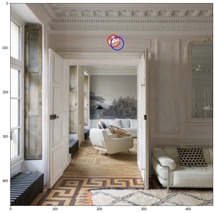
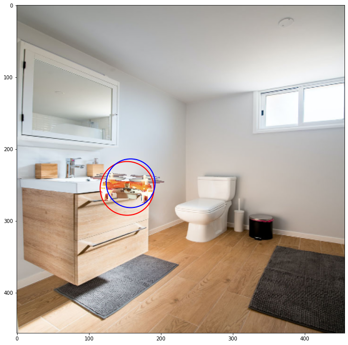
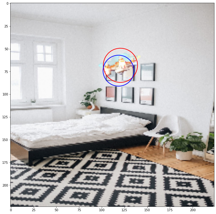
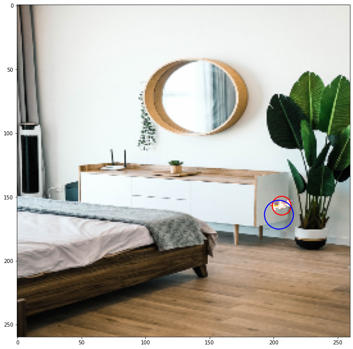
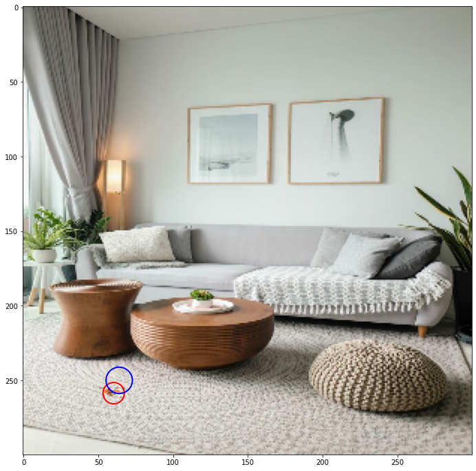
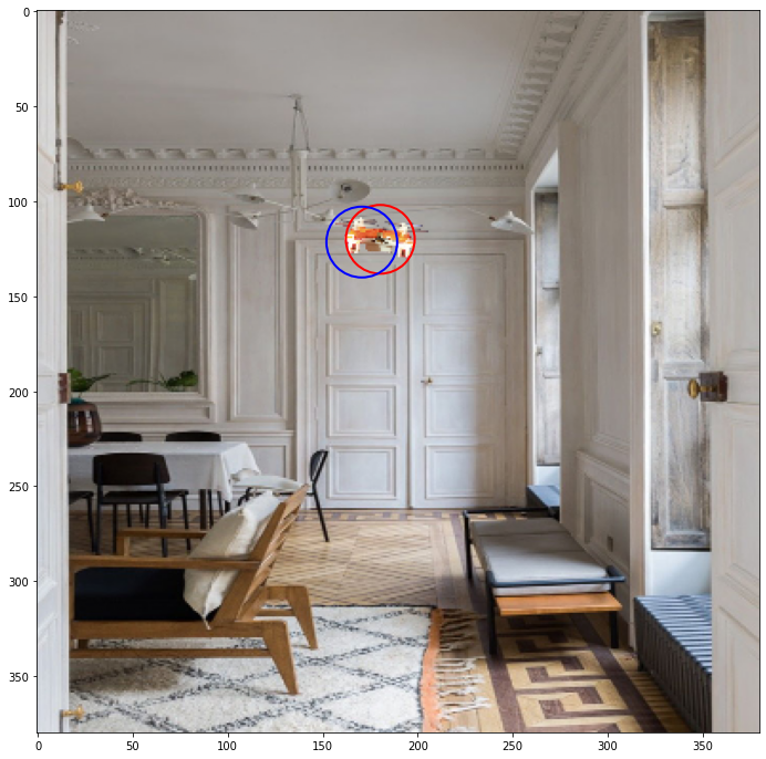
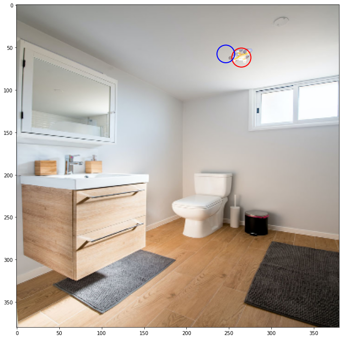
Now, test() function is for predictions and displaying results and images. It is used in our "educational" code:
# Testing on "test" part of dataset

def test(model):
  nAppartmentImageIdx = random.randint(0,
	len(arrAppartmentImageNames) - 1)
  nCopterImageIdx = np.random.randint(0,
	len(arrCopterImageNames) - 1)

  img_result, corter_center_x, corter_center_y,
	copter_radius = loadCombinedImage(
		nAppartmentImageIdx, nCopterImageIdx)
  print("GT: ", corter_center_x, corter_center_y,
	copter_radius)

  test_preds = model.predict(img_result.reshape(1,
	IMAGE_SIZE_X, IMAGE_SIZE_Y, 3))

  print("Pred: ", test_preds[0][0] * IMAGE_SIZE_X,
	test_preds[0][1] * IMAGE_SIZE_Y,
	test_preds[0][2] * (IMAGE_SIZE_X/5))

  figure, ax = plt.subplots(1, figsize=(12, 12))
  ax.imshow(img_result)

  circle_gt = patches.Circle((corter_center_x, corter_center_y),
	copter_radius, linewidth=2, edgecolor='r', facecolor="none")
  ax.add_patch(circle_gt)

  circle_pred = patches.Circle((test_preds[0][0] * IMAGE_SIZE_X,
	test_preds[0][1] * IMAGE_SIZE_Y),
	test_preds[0][2] * (IMAGE_SIZE_X/5), linewidth=2,
	edgecolor='b', facecolor="none")
  ax.add_patch(circle_pred)

  plt.show()
Finally, the "educational training" code, with "proper training" parts commented out:
INIT_LR = 2e-3
opt = tf.keras.optimizers.Adam(0.0002)

nL2 = 0.02
nDrop = 0.0 #0.2

if(bDoTraining):
  EPOCHS = 5

  model = createModel(nL2, nDrop, opt)
  model = loadModel(model, False)
  print("Model created")
  callbacks_list = getCallbacks("val_mean_squared_error",
	'min', model)
  STEP_SIZE_TRAIN, STEP_SIZE_VALID = getStepSizes()

  np.random.seed(7)
  for i in range(40):

    history = model.fit(gen_train,
      validation_data=gen_valid, verbose=1,
      epochs=EPOCHS, steps_per_epoch=STEP_SIZE_TRAIN,
      validation_steps=STEP_SIZE_VALID, callbacks=callbacks_list)

    print(nL2)
    plotFullHistory(history)

    test(model)
    test(model)
    test(model)
    test(model)
    test(model)
    test(model)

  model = loadModel(model, True)
  model.save(best_weights_filepath)    # A full model is saved


I have performed the testing with different versions of EfficientNet, from 0 to 5. The difference is in the input size they (Google) used for training.
Below, are images returned by the test() function, 3 images per each version of the net. They are zoomed to the same size, but please keep in mind that the actual size is as in the table quoted above, so B0 uses 224x224 px images and so on.
As the result, for B0 I used quadcopters that only are as small as 1/5 of the room photo. For the rest of the nets I used 1/10 as a min. size.
From the images we can see that:
1. The method does work, and it works rather well.
2. The smaller is the quadcopter image, the less the precision is: the circle around predicted position
is off and a predicted size is off as well - more than for a larger images.
3. (This is not obvious from the images) The larger the net and corresponding input images is, the
longer the training takes. Well, this was expected. What was not expected is the fact that accuracy
does not improve that much for more detailed images.
4. We can use this technology to locate quadcopters and to follow them with camera, but we probably
can not use it as is, to build the Star Wars like robotic cannon to shoot copters down - it will miss
and especially (if we use projectile weapons that have parabolis trajectory rather than a straight one)
it will give errors in size estimations. And size of a copter is a way to estimate the distance to it.
5. Then again, we can collect data from few consecutive frames and calculate a much more accurate average.
B0


B1


B2


B3


B4

B5