Proper sensor simulation

Simulating slippage

To achieve that, let's take a look at the way code worked before. In a run_localization function of kalman.py, which is a main "simulation" function, processing data in a cycle simulating the timer callback, we have to, at some point, come up with simulated sensor data. So far, we used simulated robot's state that move() function returned:

As you can see, the code is stateless, and there is no drift. To fix it, let's create two simulators, one for gyro and one for accelerometer (and one for odometry will be added later), and use them instead as the source of sensor data. Here is the code for accelerometer, code for gyro is similar:

Important note: in the code above, you can see the following comment: "Also note that acceleration is returned, but integrated velocity is stored."

Storing integrated values is one of the useful tricks, it is often applied and can (not always!) increase quality of simulation. As I understand, it is because commands we send to Kalman filter's move() are based on velocity, so if sensor reading is velocity too, it is easier for a filter to draw approximations.

As for the simulate() function, here we simply keep track of bias and add it to sensor readings. It is quite realistic.

Generally, sensor simulators take sensor parameters (mean, std_dev... - all those you can see in imu_sensor.xacro), and keep updating the inner state (coordinates, velocity, acceleration) with bias, among other things.

Note that accelerometer sensor readings that IMU returns are in robot's frame, but we store them in global frame, as our Kalman filter works in a global frame. That can be source of a great confusion.

Both accelerometer and gyroscope sensors have similar description in imu_sensor.xacro file; for each axe we have something like:

Let's see how these parameters affect the result.

Gyroscope, no drift:

First example is a gyroscope, sigma_imu_gyro is set to unrealistically large value of 0.01, and the rest of parameters (gyro_mean, gyro_bias_mean, gyro_bias_stddev) are set to zero; slippage is set to zero as well (by setting self.nSlip = ... to zero: self.nSlip = 0 in run_localization() function - this will make it ignore slippage). I am modifying code instead of passing parameters, but as it is just a single test, that will do.
This should produce the track we already saw when we worked with oversimplified code in earlier sections: the uncertainty grows, but there is no systematic error:

Accelerometer, no drift:

Same for accelerometer, again, sigma set to unrealistically large value, all other params are set to 0:

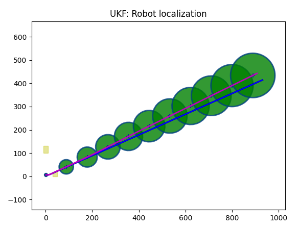
Gyroscope, bias:

Now, let's alter gyro_bias_stddev (set it to 0.0001). Gyro:

As we can see, the predicted trajectory (magenta) deviates from the real trajectory (blue). It deviates by random walk, so it can move away, then closer... at random.

Accelerometer, bias:

Gyroscope, mean:

Now let's alter gyro_mean (to 1, as well as sigma_imu_gyro, the rest is set to zero). Gyro:

Gyroscope, mean, bias:

Filally, let's provide steady deviation plus make it randomly fluctuate (sigma_imu_gyro=1, gyro_mean=1, gyro_bias_mean=1, gyro_bias_stddev=0.1). Gyro:

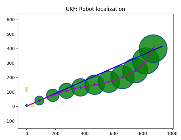
Accelerometer, mean, bias:

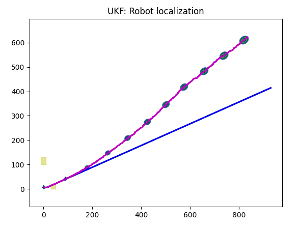
Let's summarize: sigma_imu_gyro (or _accel, depending on a sensor) sets error for a sensor. This error is zero centered. gyro_mean sets a steady drift, it is as if your gyroscope is off, not calibrated. gyro_bias_mean is the mean of the initial bias. The actual bias then evolves over time (often modeled as a random walk), but it can fluctuate, and gyro_bias_stddev sets this fluctuation.

Simulating slippage

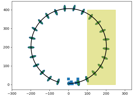
Slippage happens when our robot moves (and we do not know about it), or when we think it moves while in reality it does not. Slide downhill sideways. Hit the wall and try to drive through. Anything like that. Usually for slippage to happen we need the road to be slippery. So I am going to implement it in a very straightforward way: I am going to create rectangular areas on the surface of the world. If the robot is inside such area, it has slippage.

Rectangle on robot's trajectory:

A technical note. In run_localization() function you will find the following code:

What is going on here?

First, we set self.nSlip = 0. To understand the result, note that Kalman's move() (a model) calls getNextState() and it runs in 4 different modes, depending on the value of self.nSlip.
If 0, it simulates "perfect" world with no slippage.
If 1, it allows the Kalman filter to figure out what the slippage is. Depending on the sensor input available, results are very different, I am going to take a look at it later in this section.
if 2, the entire surface is considered slippery, which is only used to create nice looking trajectories. We do not know what slippery coefficients are in the specific place where the robot is.
Finally, if it is 3, we only model slippage in specified rectangles:

As (2) and (3) are for testing purposes only, I didn't bother to pass parameters for them, so to set our model to only consider slippage in rectangles, we need to modify the run_localization() directly:

Here, we need to set self.nSlip to either 2 (entire surface is slippery) or 3 (just rectangles are slippery). Let's set it to 3, set sensor type to GPS and run our simulation:

On the following image, robot's linear speed is *= 0.5 while driving straight in the yellow rectangle, and angualr speed *= 0.2.

What happened here? When robot entered the yellow rectangle, it was turning, so the speed of a turn dropped 5 times, see above. The linear speed dropped 2 times, so you can see the angle of turn is smaller and the length of a segment after it is smaller as well. Then there is a second turn, still within yellow rectangle, so the angle we turned is less than in a "perfect" black trajectory model. Yes, we need to look at no-slippage black line vs slippery blue one.

Now, that was modelling of movement. What about Kalman filter (magenta)? Well, it doesn't really care, because GPS provides true coordinates (same as blue line) and configuration (mostly ukf.Q) I use does not allow commands (which are not aware of slippage) to dominate over sensor data, which knows about slippage (if it is GPS).

With the values for ukf.Q set to:

... it works just fine, but this is something to keep an eye on: if Kalman filter is too confident in "command" (as oppose to GPS data), filter will try to ignore slippage.

Let's take a look at a simple example:

In this test, within a yellow rectangle, the robot moves at a straight line, so it just slows down; we can clearly see it.

Once again, as expected, GPS is not affected by slippage: no mater if real trajectory (blue) is not what filter expects (black), it still gets proper GPS signals from sattelites, so Kalman filter's output is centered around the blue trajectory.

Let's take a look at gyro sensor:

When robot enters the yellow rectangle, its linear speed drops two times (because we set it so) and its angular speed drops 5 times (getAccelerations function):

However, Kalman filter gets real values of angular velocity from gyro sensor, so at each moment of time its angular speed is correct (same as one of blue trajectory). And it doesn't get real values for linear velocity, as gyro sensor doesn't provide it. So Kalman filter will model a robot that moves with original linear speed with reduced angular speed. For this chart, we set bias to zero, to avoid distractions:

Here is the result:

First, we have black trajectory that is created by modeling the robot without friction. Doing it is only possible in simulation, as in the real world we do not have ground truth information, so it is for reference purpose only.

A blue trajectory is modelled in a similar way, but with slippage in yellow rectangle in mind. When robot enters the yellow zone, its speed drops 2 times and its angular speed drops 5 times (because this is what we hardcoded as a property of yellow rectangle). As angular speed drops more than linear, the trajectory becomes less curved. It also becomes shorter (as less distance is covered while in yellow rectangle) though it is not easy to see.

Magenta trajectory is what Kalman filter predicts. After it enters the yellow rectangle, it becomes even less curved than the blue (real) trajectory - why?
Because gyroscope doesn't know about the drop of linear speed, so Kalman filter receives info about same linear speed as was commanded (not divided by 2) and about angular speed divided by 5.

Note where the "less curved" part of this magenta trajectory ends: it runs at full speed and low angular speed until blue trajectory leaves the yellow rectangle, so it gets about as far as TWO distances blue trajectory passes in the rectangle. Because magenta trajectory entered the rectangle in the same time with blue one, and moved twice as fast until blue trajectory crossed the rectangle.

So it looks correct.

Note the lack of additional deviation from the "ground truth" black route, at the beginning, before the robot entered yellow zone. This is due to the fact that bias is set to zero value.

Let's create a trajectory where angular speed in slippery area is zero. In that case, as gyro sensor reports only angular speed, which is zero, the Kalman prediction should be close to the blue trajectory. This is exactly what we see:

Now let's take a look at accelerometer case:

In the absence of noise (almost, at such short distance) and bias, accelerometer provides Kalman filter with both linear and angular speed (first one by integrating). It means that Kalman filter has complete information and its prediction is close to real thing (magenta line is close to blue line).

Unfortunately, there is one more possible source of slippage, and people bump into it a lot as it is quite unexpected. Our robot is a 4 wheeled dif. drive one. It means that in order to turn it should rotate wheels on the opposite sides in the opposite directions. For 2 wheeled dif. drive it works fine, though if you analyse the situation for tires that have non-zero width, you will find that slippage is present even there.
For 4 wheeled one it results in slippage by design: find a video of a tank spinning in place on the grass and notice what its tracks do to a ground. The reason is that rotation is happening around the center, and points of an imaginary track (represented by 2 wheels in our case) that rotate without slippage are points in the middle. But real wheels are shifted forward and back, so they also slide sideways.

Now, Gazebo dif. drive doesn't seem to compensate for that: you tell it to rotate at 1 rad per second and it does... almost, in case of a 2 wheeled dif. drive. However if it is a 4 wheels drive (which is officially supported by Gazebo), slippage happens and rotation speed drops. And it is not compensated. And it can not be compensated, as the equation includes the friction between wheels and ground, and for a real world robot we do not have this information. Not for each point of a terrain. On the other hand, this is exactly what 4 wheeled dif. drives do in the real world, so maybe it is ok... But we still need to do localization, right?

Fortunately, in our case, it is being taken care of by the same code. Let me explain. We need slippage to be able to test our Kalman filter based navigation. If we do it and it works, then our filter is fine: it will work in the real world. Our goal is not to mimic Gazebo.

A filter implemented in kalman.py takes slippage into consideration, models it, and if sensors provide enough data, compensates for it, both in Gazebo and in the real world.

Other supported sensors

This list will grow, so it is just for reference.

GPS sensor uses simulated GPS coordinates.

odom_pos_xy sensor uses part of dif. drive's odometer functionality - coordinates (not speed). This implementation is similar to what I did with Accelerometer and Gyro, but there are things to keep in mind which I will discuss in the "Using it in Gazebo" section below.

magnet sensor is a magnetometer, it works exactly as was described in earlier sections. As magnetometer doesn't have drift, there is no reason to create a separate simulator for it.

landmarks code didn't change either. Note that Landmarks are only supported in kalman.py simulation, but not yet in Gazebo. The reason is, I haven't implemented the way for our robot to detect the landmark. There is no "landmark sensor" in Gazebo, so I need to use camera to detect Aruco markers, or to recognize signifficant points on images around, or something like that. I will implement it in later sections.

Using it in Gazebo

Let's summarize what we have so far. The Kalman filter now can take into account slippage, and sensors that should have drift, got proper simulation for it.

As the result I was able to run a realistic simulation without Gazebo, but Gazebo is still required as only there we can create a complex landscape, with obstacles, objects to move around and realistic robots. For example, my non-Gazebo simulation can model trajectory on a 2d landscape with slippery areas, but it can not model a situation where robot flips over.

Adding Gazebo is not difficult: the only thing that really changed was a new, more accurate model in kalman.py, so the rest of code should work with minimum changes.

Here are fragments of interest from Navigation.py file that implements Kalman based localization in 2d world with slippage:

Let's test Kalman localization with our sensors, one by one.

GPS:

Now, we know that black trajectory is a path modelled by the move() function in our kalman.py file. As for green path, it is a path reported by the odometer. There is no blue trajectory, as we can not simulate slippage in the "real world", but odometer (green) on a non-slippery ground should be accurate, right? Yet, black and green trajectories are very different, and the reason is...

... slippage. Yes, on a not slippery ground.

As you remember, earlier I mentioned that one of possible sources of slippage is the built-in (by design) problem with 4 wheeled dif. drive. It can not turn without its wheels slipping. Seriously. Put it on the surface that does not allow slippage, and turning will require infinite torque on wheels.

As the result, there is signifficant slippage, and it depends on the surface our robot is on. Obviously, we can not model it: who knows when robot will encounter a banana skin! So we can use odometer's linear velocity (not always, same banana skin example applies), but not angular one. Not for 4 wheeled dif. drive. Also, as odometer doesn't know anything about the real position, it can not guarantee the linear velocity as well! It can only guess.

Conclusion: we can use odometer when we drive straight, and we can not count on it when turning. Also, if road is slippery, we can not even count on it when driving straight.
Luckily, we can use other sensors to do proper adjustments.

Now, most of the bad news above only applied to 4 wheeled dif. drive. There are other designs that are less prone to that problem. Can we use those? The answer is yes.

A logical way of dealing with the problem would be to switch to Ackerman drive design, where wheels do not have to slip in order to make turn. But controlling such robot would be a more challenging task as it can not turn on the spot. Besides at this point I have to deside what is it I want my robot to do?

Ackerman drive is a logical (and probably the only logical) choice when designing a self driving car. But I would rather leave this task to Google, Cruise and General Motors. Instead, I want a low speed robot that would work on a farm, nose around on Mars or do hose cleaning.

Low speed means we do not necessarily need Ackerman drive, and "farm of house" means that most likely we will need two different robots, as the farm robot that can carry half of a ton of cargo has no place in my kitchen.

Therefore, I am going to add a 2 wheeled dif. drive robot to list of possible choices. From now on, I am not going to use odometry with 4 wheeled robot, only with two wheeled one. We can specify the type in multi_simulation_launch.py:

No other changes required! Slippage drops (yet notice that black and green trajectories are still different):

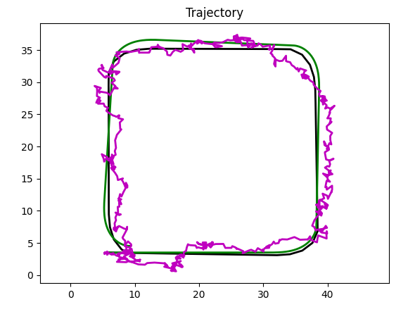
This is a small distance trajectory (a square is about 40 meters), so GPS errors and Kalman errors accordingly, are relatively high.

odom_pos_xy. This is (so far) an incomplete implementation of a Kalman filter using odometer for localization.

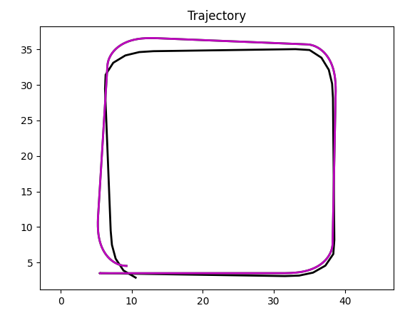
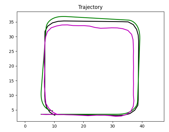
Here Kalman prediction is almost identical with green trajectory (hidden under it). If we choose longer path, differences will grow.

Accelerometer.

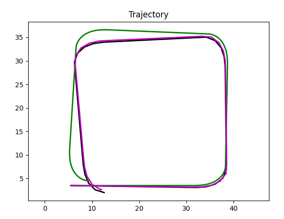
Now, this is a completely different picture. Unlike odometer, that can only count on odometry data, accelerometer "knows" real accelerations, and therefore, Kalman filter can reconstruct the ground truth (black) line.

Gyroscope.

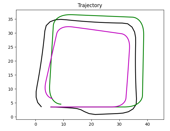
With gyroscope, Kalman filter gets "real" angular speed and "modelled" linear speed. And as there is no slippage on the linear path (in our example) and angular velocity is accurate, we can see filter producing the line close to a black trajectory.

Magnetometer.

Looks pretty much like a chart for a gyroscope, because, same as with gyro, it "knows" angular velocity and doesn't "know" a linear one. There is, however, a difference: error of magnetometer is higher, so trajectory deviates (randomly). Here is a second run under identical conditions:

Adding slippage to Gazebo simulation

So far in this section we used a non-slippery surface. The only source of slippage was a 4 wheeled dif. drive. Let's add slippage and see how our Kalman based localization handles it.

As you remember, we have already created a world with a slippery area in one of the earlier sections:

Strictly speaking, this is not 100% accurate, as tools like odometer report complete path robot travels (and the more we go up and down, the more difference is between whatever odometer reports and the change in 2d coordinates). But in that particular case the error is small.

So let's take a look at our simulation for different sensors, one by one, same as we did above, but with slippage. To do that, simply run simulation with slip.sdf, instead of empty.sdf.

An obstacle we created changes both speed (slippage) and direction of a robot.

GPS:

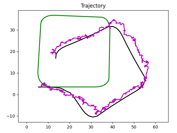
Black trajectory went sideways on an obstacle; as expected, GPS based localization followed.

odom_pos_xy:

As you can see, odometer based localization doesn't follow ground truth, as odometer knows nothing about ground truth. Instead, it follows (actually, on this picture, completely overlaps) the green trajectory, which is one reported by odometer. Do not let the accuracy of Kalman filter trick you: our localization completely ignored the slippage!

Acceleration:

Accelerometer, as opposed to odometer, "knows" the real accelerations and (by integrating) real coordinates. So it follows the black tragectory, which is ground truth.

Gyroscope:

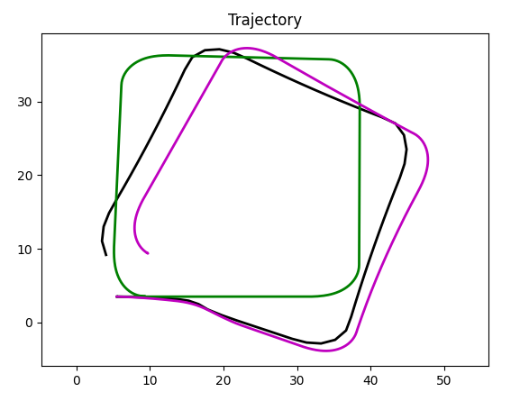
As expected, angles are correct, distances are not, so when slippage happens, model moves forward, while robot slips.

Magnetometer:

Same as with gyro, but larger errors, as magnetometer is less accurate and simulation was too short for gyro to accumulate bias related errors.

Conclusion

By now we have localization system based on a Kalman filter, that works in 2d world and can handle slippage.

Our next step is to learn to combine sensoer to perform so called sensor fusion, so that weaknesses of one sensor can be compensated by strengths of another one.