3d simulation

Availability

kalman.py file is only available to registered users, in a commercial section. If not present, you will not have access to non-Gazebo simulation, and a Gazebo simulation will use a simplified localization (in other words, it will cheat: it will use the ground truth info that you have in Gazebo and do not have in a real world, so the localization in a real world will only work if kalman.py is present).

Terrain class

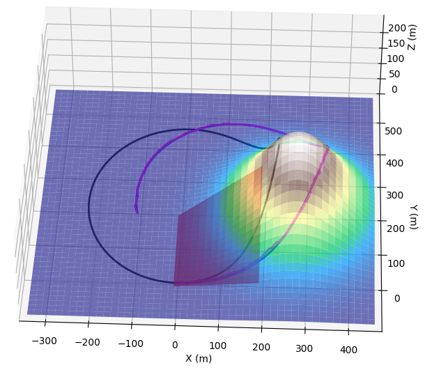
In addition to class KalmanNav, the kalman.py file now has class called Terrain. This class works with a simulated landscape: I added "Gaussian hill", tilted plane and horizontal plane, but nothing prevents you from adding more. Later, in a Gazebo section, I am going to add the code that works with DAE 2.5d landscape in the same way. Here, however, there is no difference what terrain we use to test our localization, as long as it has "hills" and "valleys", so a hill made from a 3d Gaussian "bell" seems to be a good choice.

On the resulting surface, we can draw trajectories, corresponding to ground truth path, Kalman path approximation and so on, just like we did before on a plane. Note on the picture above, "slippery areas" are reddish rectangles and black dots are landmarks: all like in our 2d simulation in earlier sections.

Accordingly, the class has only three functions the user needs to use:

Constructor:

... visualization:

... and

Obviously, constructor initializes the object of a class, for example, it sets function that is responsible for surface simulation, as well as screen size of a resulting chart and so on.

As for the surface_func, it is a function simulating the surface, in our case it will build "Gaussian hill":

figsize is the size of an image, as is done in pyplot, and resolution is a step (used internally in np.linspace). So we call it as

Visualization takes all arrays (path, slippery areas and so on) and draws them. No surprises here.

In the functions above, arrPaths is an array of trajectories (each being an array of 3d points),
arrColors are corresponding colors for these arrays,
arrSlippers is an already familiar array of slippery areas on the "Gaussian hill", we need to pass them so that they are highlited with slippersColor, same way as before, in 2d.
bShowLandmarks and landmarks determine if landmarks should be displayed, and an array of landmark coordinates.

Here is an example use of this function:

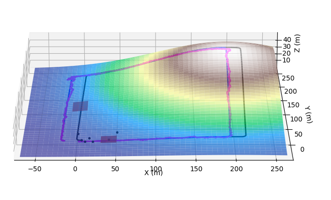
In this example we have a surface with "ideal" track that is not aware of slippage (black), ground truth track (blue) and a Kalman based trajectory (magenta). Notice few small spheres in the corner: they are landmarks. Also notice two reddish (because they are red and semi-transparent) rectangles, they are slippery areas. By the way, a true trajectory only passes through one of them.

The code is located in a kalman.py and contains a lot of comments.

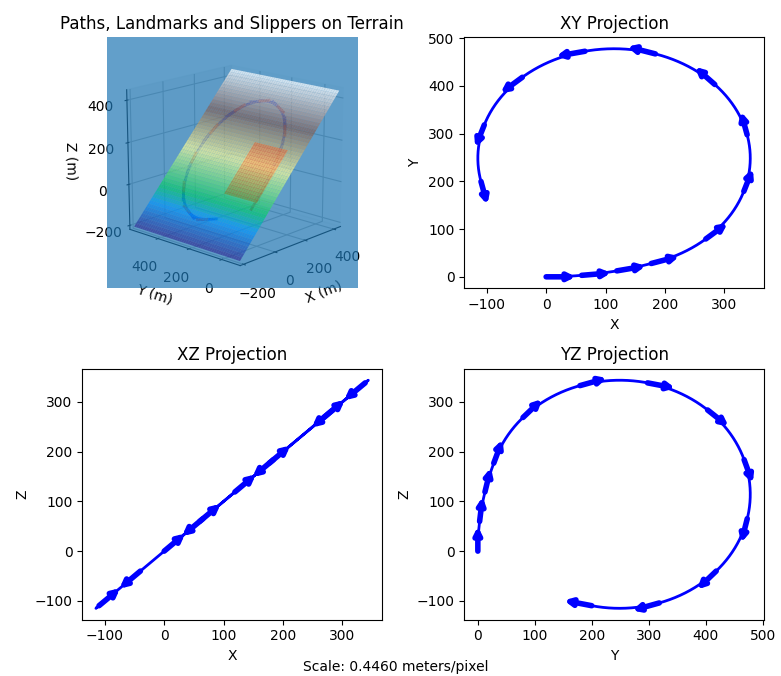
Finally, the "plot_fixed_arrow" function. See, no mater how nice 3d plot is, sometimes we want 2d projections. The user can set a flag (bShowProjections, see main() function in a code) to draw additional 2d charts, where roll/pitch/yaw of the robot are displayed as arrows. It is very convenient if something goes wrong and you need to see details: