Kalman Filter, ROS2 and Gazebo

This code is not final, I am going to gradually build the final version in few following sections while explaining what I am doing.

Let's begin with realistic GPS parameters for inexpensive GPS receiver:

Fragment of gps.xacro:

This sets standard deviation for sensor to 10 meters. But this is not the only way to influence Kalman filter's results. Meet the Q parameter.

The way we build self.ukf.Q deserves illustration. Kalman filter uses process noise, and setting it very low would be cheating. Robot will be overconfident in the model's prediction, and tend to ignore measurements.

Simulation, without ROS2, self.ukf.Q = np.eye(self.nNumOfStateParams)*0.00001

Simulation, without ROS2, self.ukf.Q = np.eye(self.nNumOfStateParams)*0.001

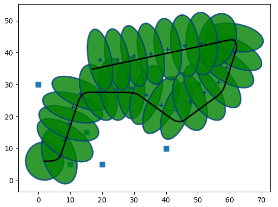
Simulation, without ROS2, self.ukf.Q = np.eye(self.nNumOfStateParams)*0.01

Also, different sensors add differently to the result, depending on their process noise, mostly, it is affected by the following: do we need to integrate them, and how many times (one for velocity, two for acceleration). As the result, instead of the code above, I had to use individual values for process noise for individual sensors:

Let's take a closer look at these values. The first value of 0.0025 in the Q matrix represents the variance of the process noise for a specific state variable: x position. The standard deviation is the square root of the variance. For a variance of 0.0025, the standard deviation is 0.05. It means that the model predicts that 68% of the measurements will fall within 0.05 m of the true value.

On unpaved terrain, the robot is likely to experience more slippage, bumps, and variations in traction. Reasonable standard deviations might be in the range of 5 to 10 centimeters (0.05 to 0.1 meters). So the value in an array above is just a reasonable estimation for a process noise.

The rest of array elements are chosen same way, based on approximate properties of inexpensive sensors. For example, The standard deviation for a gyroscope sensor typically depends on the quality and cost of the sensor. For a low-cost or mid-range gyroscope reasonable Value for Sigma 0.01 rad/s.

Here are the results for individual sensors with this process noise

GPS:

IMU accelerometer (as you can see, drift is huge; that is to be expected):

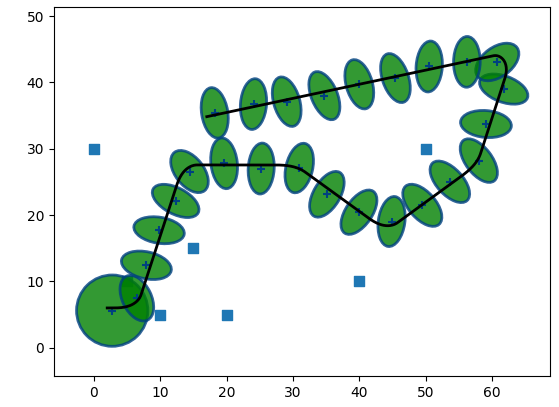
IMU gyro:

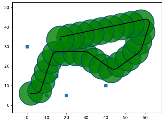
Magnetometer:

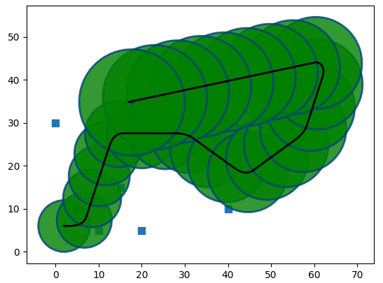
Landmarks:

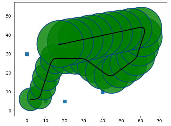
As you can see, the best results are from the sensors that do not have to perform any kind of integration (GPS, Landmarks). Other sensors have signifficant drift.

Also, as was mentioned in the intro to this section, currently you can not combine sensors, at least some of them. For example, GPS doesn't have drift, but IMU does, and there is no way to adjust for it. Well, no way now, I am going to address this issue in the next section.

In the same time, we can use GPS and Landmarks together, as they have no drift and are therefore compatible:

Can we use IMU acceleration or gyro with magnetometer? Probably not, as they can drift in different directions, and it is not taken care of yet. I will address that later.

I have also added two worlds: one "empty.sdf" to model robot in 2d space, and one "slip.sdf", that has a slippery area to model wheel slippage.

Now, this was all about a rather primitive "simulation" I created for my Kalman filter. It doesn't care for sensor drift, it doesn't model robot's vibration and magnetic fields... It is a proof of concept and nothing more.

To do a proper simulation we either need a real robot, or a model of such in a good physics simulator. Currently I use Gazebo. Physics simulator? Yes. Good? Let's take a look at accelerometer simulation:

Looks like accurate trajectory with some random jumps (including the initial one when we lost direction).

After some pain and suffering, I found that:

1. Gazebo runs at 10 Hz. This is a default value. And if you ignore it and try something like this (imu_sensor.xacro):

... then you are in for a disaster. If you want to have sensor at 100 Hz, you need to explicitly run Gazebo at 100 Hz (or more), too (multi_simulation_launch.py):

Now we have "publish_rate" set to 100 Hz, otherwise we get garbage 9 times out of 10.

Alternatively, we can set both Gazebo and sensor to 10 Hz, but that means our IMU will run much slower than it would be in a real world. The reason it matters is, GPS usually runs at 10 Hz, and 100Hz IMU can fill in gaps... which will not happen if they work at the same frequency.

So let's set simulation to 100 Hz:

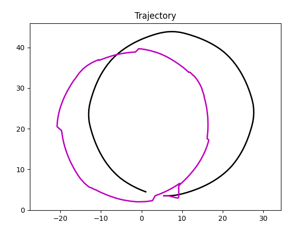
Ugly. What is wrong this time? Simulation. Gazebo runs at default 50 or 40 "steps" of a simulation and this is not enough to produce good results for accelerometer, at least not in my robot.

Can we use moving average? Let's try, after all, if we have 100Hz, we can apply EMA with period 10, right (Navigation.py)?

Still ugly, which is not a big surprise: data is wrong, not noisy. What can we do?

The way simulation works, it performs certain steps, and the smaller step, the higher the accuracy is. Unfortunately, at some point simulation will begin to slow down, so it is definitely not a cure. But it works:

empty.sdf, before:

empty.sdf, after:

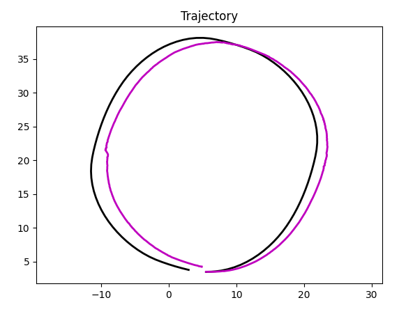
As I mentioned, even for a simple robot model like one I use, on a very good PC, simulation speed is at its limit. Add another robot, and it will slow down. An obvious solution is to go back to 10 Hz, which I might do after I am done with sensor fusion.