Home
Tutorials
Code structure - Important!
An important info about the structure of the code.
The code is divided in two sections: open access and by subscription
The first part of the code for this section is located both in landscape_designer
part of an archive
Note that in addition to landscape_designer, the archive includes some additional folders,
like maps and worlds, that are used by all projects
and therefore are located outside of them. An archive has proper directory structure, so all you have to do
is expanding it.
Also note that currently the ROS2 Humble is used. However, older sections of this tutorial
still use Galactic and maybe some older versions. I will fix it in future.
For installation instructions, see Installation.
As for the second part: the tutorial is divided in two parts, too. First part is about
the theory, it is complete and free (see below).
The code itself however has either free access, or by subscription, like some utilities that
live in "utils_commercial" folder. When you try to access these utilities, you will be asked to
log in.
Additionally, Kalman part of that code is moved to a by-subscription section as well:
kalman_nav.zip.
Note: This archive should be added to same folder where you have unpacked
archive.
Let me explain how Kalman code works and why do you need commercial code if free code works
just fine.
A kalman.py file was moved to by-subscription section and therefore will not be
available unless you get it and copy it over to nav25d_06/nav25d_06 (or later) folder.
The (free) Navigation.py file checks if this file is
present and either uses it (in which case you will get a complete Kalman based
localization) or not (in which case Kalman filter is replaced with a rather
primitive simulation).
As the result, in a Gazebo simulator, all future demos will work even without
by-subscription files. But of course, in a real world your robot will not have
these localization abilities.
Important note: as I write more sections, the kalman_nav.zip file will
get additional context. Once purchased, it gives you 1 year of access, so when,
for example, I add support for aruco markers in Gazebo (available already) or make the
navigation to respect the fact that the world is round, or whatever else related
to localization - it will go to this archive and will be available with the
same subscription. Unless this project is terminated, of course.
As for utilities that are available from by-subscription section, they do not affect simulation,
but give you tools to design the world, control robot in a simulation and provide some other
nice-to-have features.
An important info about the structure of the code.
The code is divided in two sections: open access and by subscription
The first part of the code for this section is located both in landscape_designer part of an archive Note that in addition to landscape_designer, the archive includes some additional folders, like maps and worlds, that are used by all projects and therefore are located outside of them. An archive has proper directory structure, so all you have to do is expanding it.
Also note that currently the ROS2 Humble is used. However, older sections of this tutorial still use Galactic and maybe some older versions. I will fix it in future.
For installation instructions, see Installation.
As for the second part: the tutorial is divided in two parts, too. First part is about the theory, it is complete and free (see below).
The code itself however has either free access, or by subscription, like some utilities that live in "utils_commercial" folder. When you try to access these utilities, you will be asked to log in.
Additionally, Kalman part of that code is moved to a by-subscription section as well:
kalman_nav.zip.
Note: This archive should be added to same folder where you have unpacked
archive.
Let me explain how Kalman code works and why do you need commercial code if free code works just fine.
A kalman.py file was moved to by-subscription section and therefore will not be available unless you get it and copy it over to nav25d_06/nav25d_06 (or later) folder. The (free) Navigation.py file checks if this file is present and either uses it (in which case you will get a complete Kalman based localization) or not (in which case Kalman filter is replaced with a rather primitive simulation).
As the result, in a Gazebo simulator, all future demos will work even without by-subscription files. But of course, in a real world your robot will not have these localization abilities.
Important note: as I write more sections, the kalman_nav.zip file will get additional context. Once purchased, it gives you 1 year of access, so when, for example, I add support for aruco markers in Gazebo (available already) or make the navigation to respect the fact that the world is round, or whatever else related to localization - it will go to this archive and will be available with the same subscription. Unless this project is terminated, of course.
As for utilities that are available from by-subscription section, they do not affect simulation, but give you tools to design the world, control robot in a simulation and provide some other nice-to-have features.
Introduction
Earlier (much earlier) I had sections explaining how to use Path Planners and Path Follower in Nav2 ecosystem. As most of this ecosystem is for 2d world, it will not work in our 2.5d case, so we need to come up with the code of our own. Another reason we want to do it is, Nav2 is relying on 2d lidar way too much: tilt your robot and you are in trouble.
So in this section the custom UKF code and custom path planners (but not followers yet!) are combined, so that robot can figure out its position and plan the path to some goal point - across the rugged terrain with some areas that are good for driving and some that should be avoided.
Also, in this section I will begin altering the code structure, so that resulting app is more structured and can run on multiple computers. See, some path planners can require resources, and sometimes we do not want to make our robots too smart. By controlling them from a centralized server, we can save money by not installing Intel+video card where a simple Pasp PI or even Arduino will do.
But for that we need to be very careful with what code runs on a robot, which code runs on a server, and what the robot should do if a server is temporary unavailable. So I am going to move the functionality between nodes, in order to make the code more modular.
Note that it is the first publication about "path planners", the following section will finalize both the code and a functionality. It means that, as usual, I am taking the "tutorial" approach, rather than providing a final - and harder to understand - result.
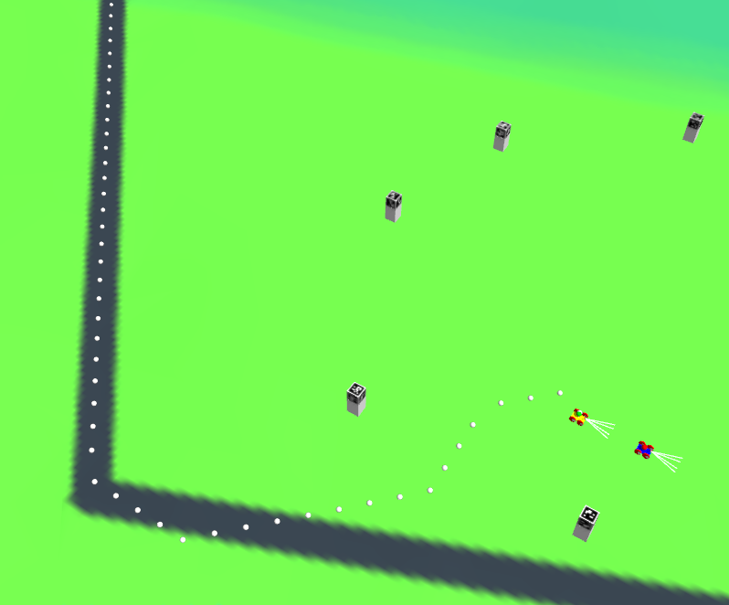
On the following screenshot you can see two robots with two pathes. Note that a path looks like a zigzag, which is understandable: it goes from one cell of a grid to another (A* Grid algorithm). I will address smoothing in later sections, and also in this section I will present Dynamic Cell Size A* Algorithm that is way better than a vanilla A* Grid.