Sensor fusion in 3d world (no Gazebo)

What if we have no sensors?

Yes, we can do some localization with no sensors. After all, we still have our commands, so we know our expected linear and angular velocities. Of course, our robot will be totally unaware of slippage, plus Kalman filter uses a model, and it has process noise that will not be corrected during an update step, as there are no sensors to base this update on.

So we will have a growing error:

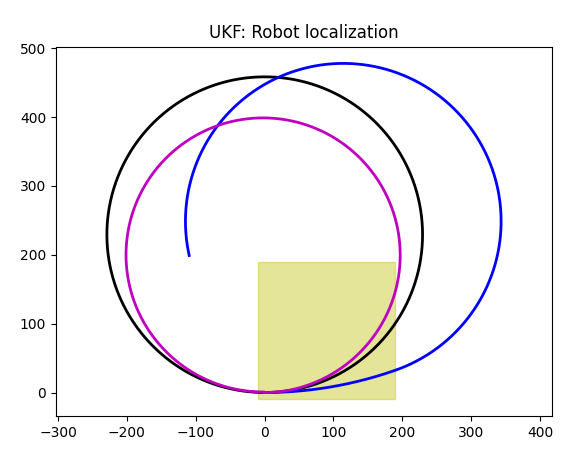
Here, black trajectory is a slippage-free one, blue trajectory is one with slippage. In the previous section I have explained the way it works, and I will revisit it later in this section.

As for a magenta trajectory, it is a one built by Kalman filter. As you can see, robot is lost, though trajectory doesn't look random: I would say the error is constant, either in angular velocity, or in linear velocity, or both. I do not see any reasons to investigate what happens here, but it can be done if necessary.

The way it works, we apply UKF's "predict" step, add process noise, and do nothing for an update, one time after another. So the error gets higher.

GPS

I have updated GPS sensor to handle 3d coordinates (by adding zPos to robot's state vector), and it now works in 3d, no surprises here:

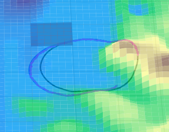
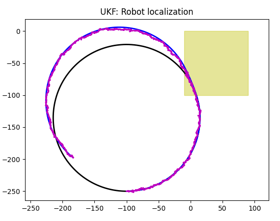
Interesting enough, UKF seems to be able to catch proper robot orientation at some point, though I would not count on it:

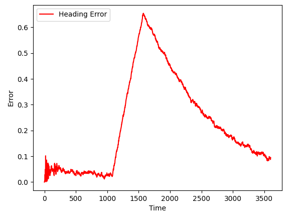
As for position error, it is very good, way better than 10 meters we set as a GPS error for a simulation:

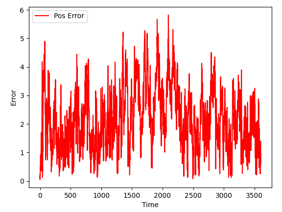
Let's take a look at trajectory produced by a simulation. It is very important to understand what is going on here, as if we add new sensors, we will need a way to make sure our localization works properly:

As you can see, robot moves across slippery areas while on the linear part of its trajectory: angular velocity is zero. According to our simulation, linear velocity drops when on slippery areas, you can see it on a blue trajectory.

Now let's take a look at first (of three) simulations again:

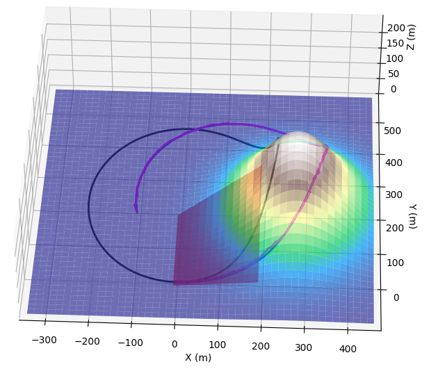
As I mentioned, GPS sensor doesn't add errors if slippery area is encountered. This is because it takes "true" coordinates (plus some error of course) as opposed to doing "dead reckon" as inertial sensors do. On a chart, it means that GPS based Kalman prediction follows the blue line (real path of a robot) as opposed to following black path that is unaware of slippage. Slippage in a trajectory above happens once, when the blue path crosses the bottom slippery rectangle. At that point the speed drops twice (we hardcoded it in a simulation for slippery areas), while angular speed drops 5 times. So the a blue trajectory goes left to right with less curvature than black trajectory does.

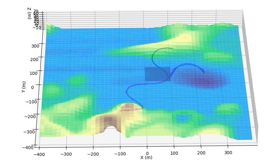
As soon as blue trajectory is out of slippery area, it draws the rest of a circle same way black trajectory does, so we see it shifted to the right. Here is another simulation that makes it even more clear:

Accelerometer

Accelerometer "knows" about both linear velocity, as acceleration can be integrated into speed and at tracking rotations. Note however, that to reduce errors (unless we want to write extra code to compensate it), we need to place accelerometer in the robot's center of rotation. This way, when robot rotates in place, it does not register "false" linear acceleration.

Here is the output of our localization code that uses acceleration only. It looks ok, except, of course, it will add more errors as time passes, unless we correct it. As a correction, GPS sensor can be used (see later in this section for GPS + accelerometer results).

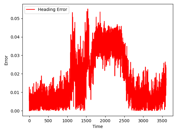
Also note that heading estimation is very accurate (on the chart, heading error is in radians, not degrees).

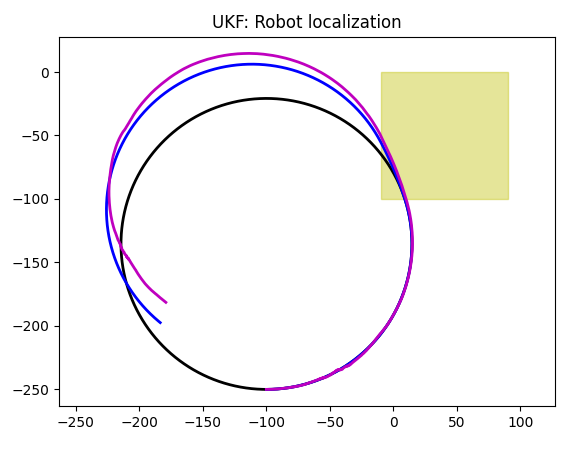
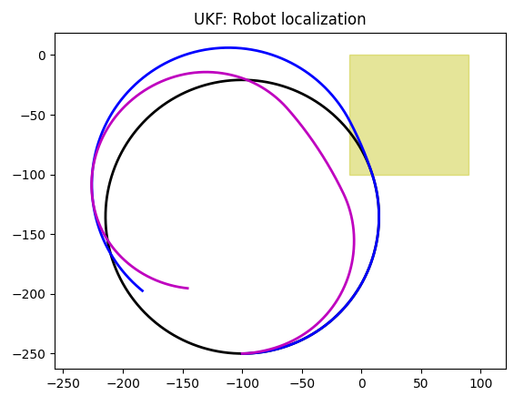
The chart above is interesting. Not only accelerometer based Kalman filter followed linear parts of a blue line, but it also turned at the right angle. How?

To explain what I mean, look at a yellow rectangle that marks slippery area. A segment of a blue line (one between two turns) that is in that rectangle is two times as short as a corresponding segment of a black line, as we set (see kalman.py code) that speed drops 2 times in the slippery areas. But that created a situation when the turn (at the right-top part of a yellow rectangle) also happens inside a slippery area. And in our code, speed of turn on slippery area is set to be 5 times smaller. You can see blue line turns very little, compared to a corresponding part of a black line. Yet, magenta line, a Kalman-based prediction follows the blue line in that: it makes a less of a turn. Which means our accelerometer is aware of turns, right?

The answer is, if our robot rotates in a spot, accelerometer, which is located in its center of rotation, will show nothing. But our robot rotates around a center that is outside the robot, by a large arch. That creates centripetal force which accelerometer can detect.

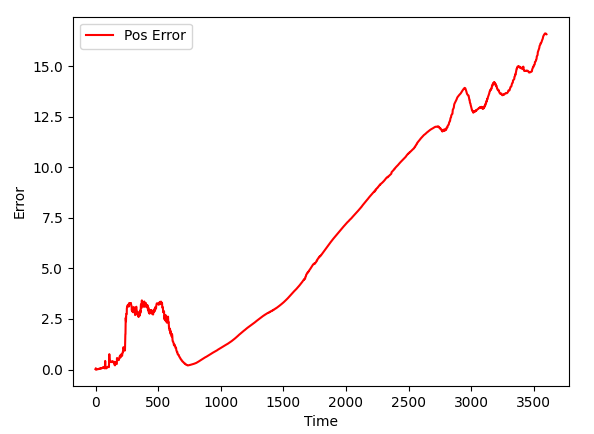
Position error is very small too, and as expected, it increases with time:

Let's make it more obvious: let's run same circle, 100 times. To do so, in a main() function, let's modify the code:

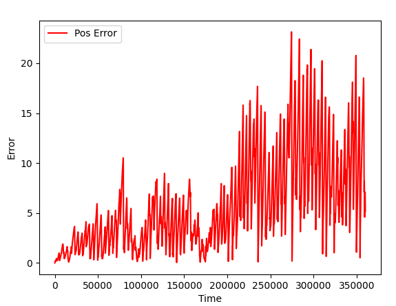
As expected, position error increases with time, as we run 100 circles in a row.

Gyroscope

Gyroscope knows nothing about position, so the position drifts. To understand this, let's ask ourselves, what gyroscope returns? It gives us heading, right? Does knowing heading helps to figure x and y coordinates? It does, as our setup uses orientation when computing coordinates, but the emphasize will probably be on heading. In other words, UKF will sacrify coordinates to get better heading accuracy. As for the heading itself, it is quite good:

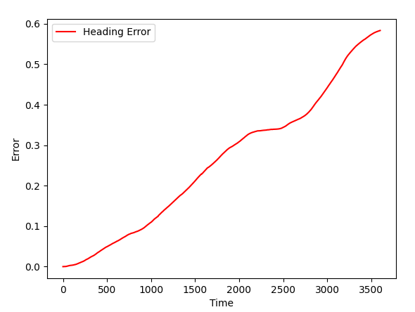
Let's take a look at how the accuracy of a GPS sensor affects the result. Current settings are for the inexpensive cheap model. Let's purchase a better gyroscope for our project (note that I have commented our old values and added ones that are improved two degrees of magnitude):

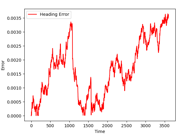
Can we use it? Of course. Having accurate heading and lilear speed will allow us to improve the overall accuracy in coordinates, this is exactly what sensor fusion is for.

Magnetometer

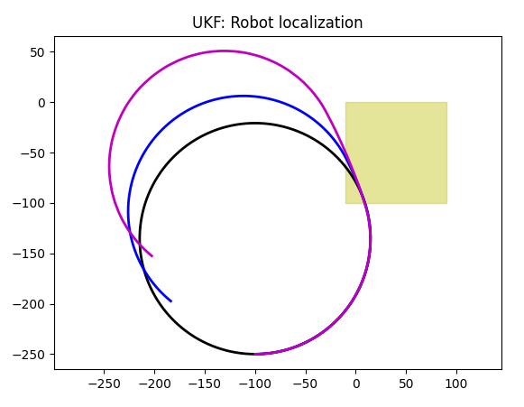
As you can see, we can not rely on coordinates with magnetometer, but we can rely on a turn angle. The obvious difference between gyroscope and magnetometer is due to the fact that gyroscope reads angular velocities, and Kalman filter has to perform integration... which introduces errors. Again, in custom setup, if we know exactly how our particular robot works, it can be fixed. I will talk about it in later sections.

We already saw a similar picture in a 2d section earlier. The blue line turns less while in a slippery area, and robot (that leaves blue line behind) also moves slower there. In the same time, magnetometer can detect the "turns less" fact, but can not detect the "moves slower" one, so the rotation speed is less, but the linear speed is taken from a control command, as the result, we get magenta line that is different from blue one.

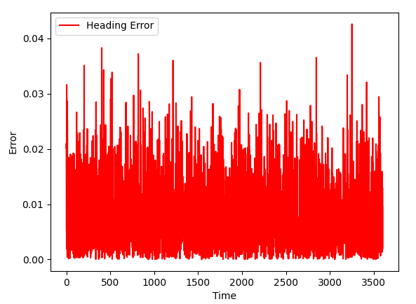
As should be expected, the heading is very accurate:

Odometer

I mentioned it before, let me repeat. Odometer doesn't know anything about landscape. It counts wheel rotations, as if it was on a flat surface. Imagine the robot going straight (no turns) and up the slope at a tilted plane, along X axe. Actual x coordinate will be a projection of the linear robot's path to the horizontal plane. Which is path_length * cos(alpha). While robot's x coordinate according to odometry will be path_length.

Odometer also knows nothing about slippage.

And that reminds us the "command" we use to control te robot. It also believes that robot moves on a horizontal plane, and it is also not aware of slippage. So... why use odometry?

First of all, odometry can be used if we do not have access to commands.

Second, it can be used if commands are not the only reason for a robot to move. For example, we accelerate, and then let the inertia to carry robot forward, until friction stops it.

Or we can turn off the engine and let robot to drive down hill using gravity.

How to use odometry? A proper way would be to adjust distance reported on every step by the angle robot is at, so that the projection to a horizontal plane described above is compensated properly. That means we need to have other sensors or, better, to have Kalman filter with these other sensors run, before we fix odometer data. It means we have to know the exact robot's design and to abandon the goal of this tutorial, which is to "merge any combination of sensors".

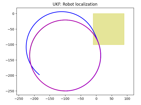
As you can see, odometer based Kalman filter accurately models the path that ignores slippage. This places another limitation on odometer: we only use it on a surface with great friction.

Landmarks

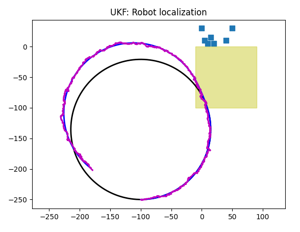
Landmarks work as well as they were in a 2d world, no surprises here:

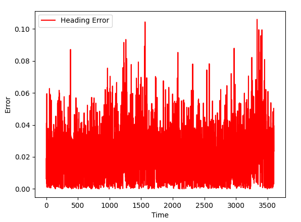
Orientation info is accurate, too:

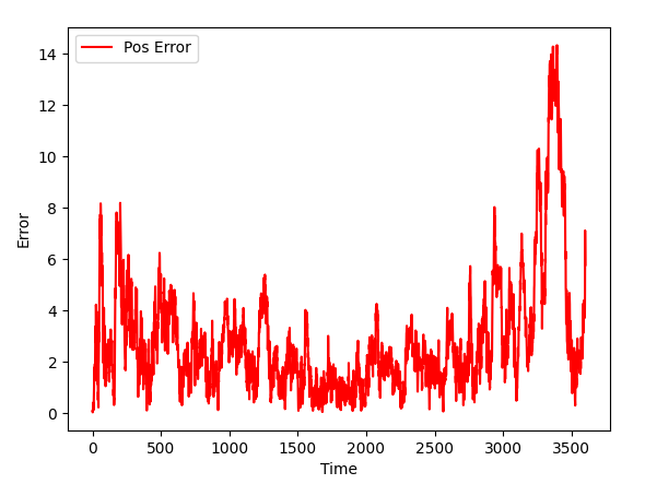
As expected, the further we are from landmarks, the higher is an error:

GPS + Accelerometer

GPS	Accelerometer + GPS

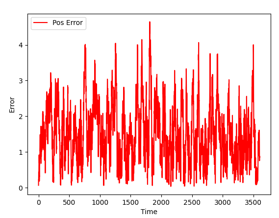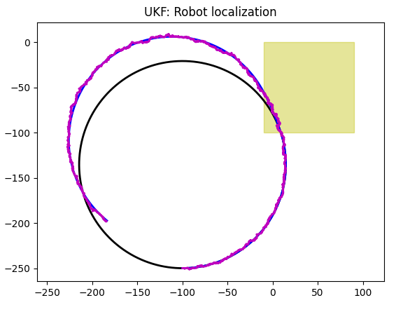
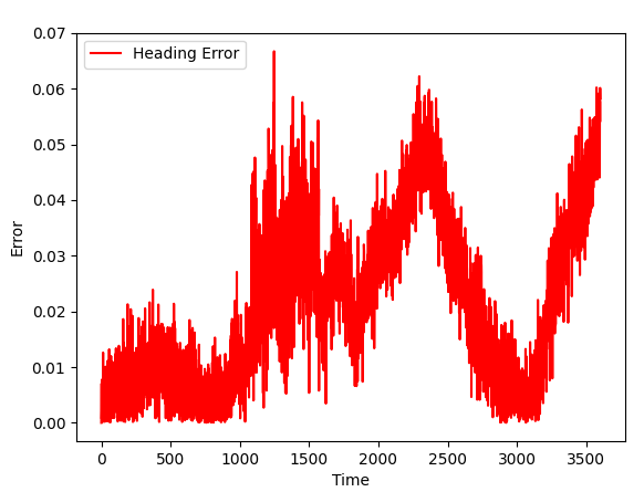
As Kalman filter got new data (and data can be used in the content of a task), the quality of a simulation improves. We now have good orientation accuracy and slightly improved position accuracy.

GPS + Gyroscope

GPS	GPS + Gyroscope

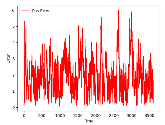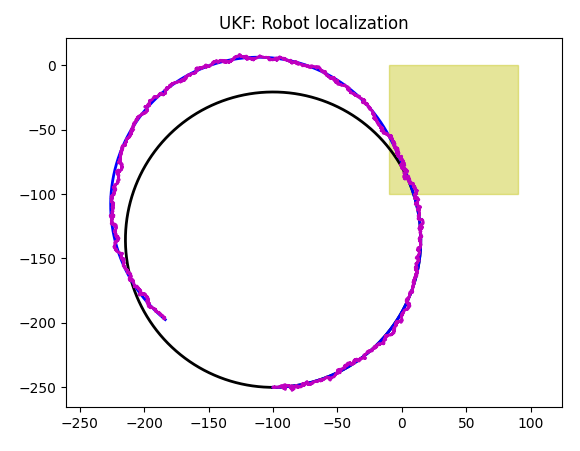
As Kalman filter got new data (and data can be used in the content of a task), the quality of a simulation improves. We now have good orientation accuracy and slightly improved position accuracy.

GPS + Magnetometer

GPS	GPS + Gyroscope

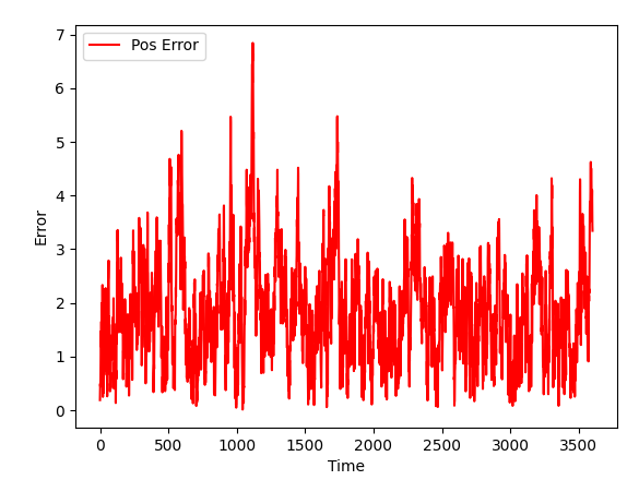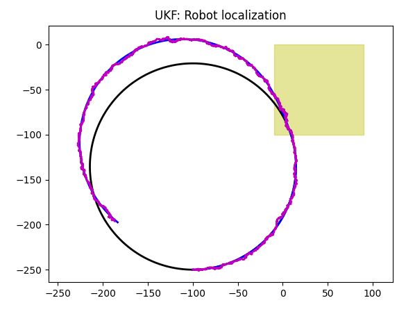
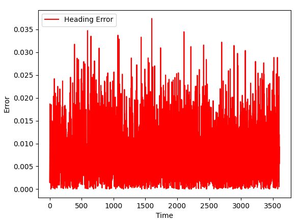
As Kalman filter got new data (and data can be used in the content of a task), the quality of a simulation improves.

GPS + Odometer

As you saw above, adding a second sensor to GPS improves accuracy. However, that does dot apply to odometer in the form it is implemented here:

GPS	GPS + Odometer

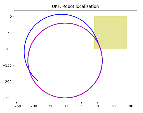As you can see, GPS sensor is ignored, and odometer based Kalman filter models the trajectory that is unaware of slippage. The reason of "ignored" part is the way Q vector of Kalman filter is configured, and it can be changed. However in that case we will get a weighted average of some kind, as Kalman filter can not model two different trajectories at once. I have already explained the reasons odometer ignores slippage and Z coordinate and the way it should be fixed.

Accelerometer + GPS + Gyroscope

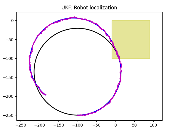
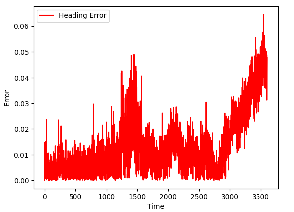
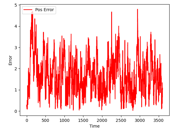
As more sensors are added, we see further improvements.